Bayesian and Frequentist A/B Testing

Some notes on A/B Testing, the frequentist and Bayesian approaches, and their differences.

NoteTLDR

Sources for inspiration:

• Is Bayesian A/B Testing immune to peeking? Not exactly
• How Not to Run an A/B Test

The Peeking Problem

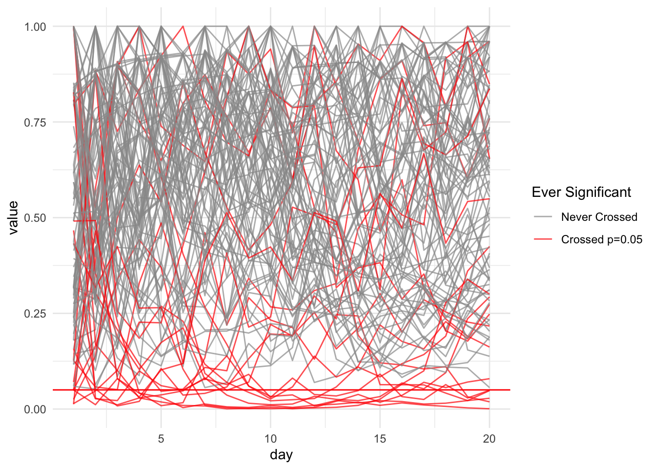
Say you are a data scientist running an A/B test on a new feature. Let’s say you run this experiment for 20 days, and on each day get 10,000 samples. Further, suppose that the groundtruth is that for both version A and version B, the clickthrough rate¹ is 0.1%. We can simulate the total number of clicks during a single day as following a Binomial distribution \(B(n = 10000, p = 0.001)\)².

¹ A typical definition for Clickthrough rate (CTR) is clicks \(\div\) impressions (number of times the ad is shown). See this page for details.

² … for simplicity assume the 20 Binomial distributions are independent from each other

Let’s say we use the Chi-squared two sample proportion test.

# set random seed 
set.seed(57)
# simulate daily clicks 
clicks_A_daily <- rbinom(20, size = 10000, prob = 0.001)
clicks_B_daily <- rbinom(20, size = 10000, prob = 0.001)
# calculate cumulative clicks 
clicks_A_cum <- cumsum(clicks_A_daily)
clicks_B_cum <- cumsum(clicks_B_daily)

impressions_cum <- (1:20) * 10000

# loop and calculate p-value for each day 
p_values_cum <- numeric(20)

for (d in 1:20) {
  k_A <- clicks_A_cum[d]
  k_B <- clicks_B_cum[d]
  n_total <- d * 10000
  
  observed_data <- matrix(
    c(k_A, n_total - k_A,
      k_B, n_total - k_B), 
    nrow = 2, 
    byrow = TRUE
  )
  
  test_result <- chisq.test(observed_data, correct = FALSE)
  
  p_values_cum[d] <- test_result$p.value
}

# p_values_cum

Plot.plot({
  y: {grid: true},
  marks: [
    Plot.ruleY([0.05], {stroke: "red", strokeDasharray: "5,5"}), 
    Plot.line(transpose(day_data), 
      {x: "day", y: "value"}, 
      { stroke: "black" },
    ), 
    Plot.dot(transpose(day_data), 
    {x: "day", y: "value"}, 
    { fill: "black" },
    )
  ]}
)

If we peeked at the p-value during the data collection process, before the 20-days run up, and then decided to stop collecting data on day 3 or day 4, then we probably would never realize that in the long run, the p-value is not statistically significant.

---

We can repeat the above experiment for 100 times:

# define function for simulation 

clicks_A_all <- matrix(rbinom(20 * 100, size = 10000, prob = 0.001), nrow=100, ncol=20)
clicks_B_all <- matrix(rbinom(20 * 100, size = 10000, prob = 0.001), nrow=100, ncol=20)

sim_one_day <- function(i){
  # simulate daily clicks 
  clicks_A_daily <- rbinom(20 * 100, size = 10000, prob = 0.001)
  clicks_B_daily <- rbinom(20, size = 10000, prob = 0.001)
  # calculate cumulative clicks 
  clicks_A_cum <- cumsum(clicks_A_daily)
  clicks_B_cum <- cumsum(clicks_B_daily)
  
  impressions_cum <- (1:20) * 10000
  
  # loop and calculate p-value for each day 
  p_values_cum <- numeric(20)
  
  for (d in 1:20) {
    k_A <- clicks_A_cum[d]
    k_B <- clicks_B_cum[d]
    n_total <- d * 10000
    
    observed_data <- matrix(
      c(k_A, n_total - k_A,
        k_B, n_total - k_B), 
      nrow = 2, 
      byrow = TRUE
    )
    
    test_result <- chisq.test(observed_data, correct = FALSE)
    
    p_values_cum[d] <- test_result$p.value
  }
  
  p_values_cum %>% as_tibble(.) %>% 
    mutate(day = 1:20, 
           exp_id = i)
}

total_sim_df <- data.frame()

for (i in 1:100){
  total_sim_df <- rbind(total_sim_df, sim_one_day(i))
}

Warning in chisq.test(observed_data, correct = FALSE): Chi-squared
approximation may be incorrect

total_sim_df <- total_sim_df %>% group_by(exp_id) %>% 
  mutate(ever_sig = any(value <= 0.05)) %>% 
  ungroup(.)

total_sim_df %>% group_by(ever_sig) %>% count(.)

# A tibble: 2 × 2
# Groups:   ever_sig [2]
  ever_sig     n
  <lgl>    <int>
1 FALSE     1620
2 TRUE       380

total_sim_df %>% ggplot(aes(x = day, y = value, group=exp_id, color = ever_sig)) + 
  geom_line(alpha = 0.7) + 
  scale_color_manual(
        name = "Ever Significant",
        values = c("TRUE" = "red", "FALSE" = "gray60"),
        labels = c("TRUE" = "Crossed p=0.05", "FALSE" = "Never Crossed")
    ) +
  geom_hline(yintercept = 0.05, color = "red")

Note that the above example is adapted from [how not to run an A/B test].

Anyways, the promise that the frequentist paradigm is making is that it helps control the type I error. When executed correctly. Bayesians don’t help with this.

If we do want to do things correctly and not let’s say, run an experiment for an indefinite amount of time, another thing to do is to implement (frequentist) sequential Bayesian testing correctly.

Does Bayesian A/B Testing solve the problem of peeking³?

The short answer is not necessarily. See explanations here and here.

# code-fold: true 
# test to see if this is right ... 
chisq.test(matrix(c(127, 5734 - 127, 
  174, 5851 - 174), nrow=2, byrow= TRUE))

    Pearson's Chi-squared test with Yates' continuity correction

data:  matrix(c(127, 5734 - 127, 174, 5851 - 174), nrow = 2, byrow = TRUE)
X-squared = 6.2957, df = 1, p-value = 0.0121

There is also this research paper on optional stopping in Bayesian testing.

³ aka “optional stopping”

Bayesian A/B testing with an example.

NoteSources

• this blogpost from Kaggle that uses PyMC.
• Another blogpost from Kaggle that does not use PyMC …? but uses statsmodels instead (and plotnine …? did not know plotnine is a thing for 6 years ago …)
• this paper by people at Apple.
• this blog post
• this official tutorial from PyMC.

If you look at the first formula for binary outcomes, it says that when the prior is uninformative (i.e., uniform, alpha = beta = 1), then the updated posterior is …? So in a sense, a beta distribution is a very special kind of distribution⁴ that allows closed-form calculations of updated posterior I believe …

⁴ conjugate prior

Beta distribution

viewof mu = Inputs.range([-10, 10], {value: 0, step: 0.1, label: "Location (mu)"})
viewof sigma = Inputs.range([0.1, 10], {value: 1, step: 0.1, label: "Scale (sigma)"})
viewof lambda_val = Inputs.range([-5, 5], {value: 0, step: 0.1, label: "Skew (lambda)"})
viewof nu = Inputs.range([1, 100], {value: 10, step: 1, label: "Degrees of Freedom (nu)"})

Some reflections

I think the real thing underlying all of this is that they each contain their baked in assumptions, and it is important that we know which assumptions to use and which not to use.