Hierarchical modeling with PyMC and brms

NoteTLDR

To bridge the gap between R-based research and Python-based deployment, I compared an end-to-end Bayesian workflow using PyMC + ArviZ against the brms + tidybayes + ggplot2 stack. To make my examples concrete, I utilized the reedfrog and chimpanzee examples from McElreath’s Statistical Rethinking.

Certain things stood out to me:

• brms abstracts away the “boilerplate” (e.g., dummy coding, index variables, non-centered parameterization) that one still needs to implement manually in PyMC.
  
• Nevertheless, PyMC forces users to explicitly define the data generating process starting from the hyperpriors, and shares a closer resemblance to the underlying mathematical equations of the model. brms on the other hand, folds a lot of writing intos its formula, which could take a while to get used to, and does not make the process of specifying priors easy. PyMC also makes specifying multilevel models easier.
• arviz introduces a more sematic way of handling data (via xarray and InferenceData), but the R ecosystem remains the superior option for visualizing data in tidy format. Grammar of Graphics makes the process of creating custom prior and posterior plots intuitive.
  • arviz is also currently undergoing some refactoring changes (per this article), and some of the plotting functions don’t quite produce the results that those who are familiar with bayesplot would expect them to look like. So technically one also need to look into arviz-plots in addition to the base arviz. plotnine, while powerful and uses grammar of graphics, does not support tidybayes geoms as of now.

All this is to say, for a researcher used to R’s high-level abstractions, the Python transition currently feels very painful — the potential for production integration is definitely there¹, but the developer experience is significantly more high-friction.

I also recommend reading [this post](https://discourse.mc-stan.org/t/how-to-translate-between-pymc-and-stan/38574 and this post for people interested in the differences (as well as how to trasnlate) between PyMC and Stan.

¹ e.g., via pymc.ModelBuilder

Tadpole survival

We will use the tadpole survival in ponds dataset used in McElreath’s Statistical Rethinking textbook. The reedfrogs.csv is obtained from here. One can follow along the original textbook starting from Chapter 13.1 Example: Multilevel tadpoles.

First we load the necessary libraries and data:

R

set.seed(51)
library(tidyverse)
library(ggplot2)
library(brms)
library(here)
library(bayesplot)
library(tidybayes)
theme_set(theme_minimal())

df <- read.csv2(here("posts", "pymc-hierarchical", "reedfrogs.csv")) %>% as_tibble(.)
df %>% head(5)

# A tibble: 5 × 5
  density pred  size   surv propsurv
    <int> <chr> <chr> <int> <chr>   
1      10 no    big       9 0.9     
2      10 no    big      10 1       
3      10 no    big       7 0.7     
4      10 no    big      10 1       
5      10 no    small     9 0.9     

Python

import pandas as pd
import os 
os.environ["PYTENSOR_FLAGS"] = "cxx="
import pymc as pm
import pytensor
import arviz as az
import arviz_plots as azp 
from pyprojroot.here import here 
az.style.use("arviz-docgrid")

df = pd.read_csv(here("posts/pymc-hierarchical/reedfrogs.csv"), delimiter=";")
df.head(5)

   density pred   size  surv  propsurv
0       10   no    big     9       0.9
1       10   no    big    10       1.0
2       10   no    big     7       0.7
3       10   no    big    10       1.0
4       10   no  small     9       0.9

We will focus on the number surviving (surv) out of an intial count (density).

No pooling

Tip

Note that for this particular example, each row is its own tank.

Math model:

\[ \begin{align} \texttt{surv}_i &\sim \text{Binomial}(\texttt{density}_i, p_i) \\ \text{logit}(p_i) &= \alpha_{\text{TANK}[i]} \\ \alpha_j &\sim \mathcal{N}(0, 1.5), j \in [48] \end{align} \]

The first step is to specify the model, specify the priors, and perform a prior predictive check:

R

We use the bf function in brms to set up the model formula:

df <- df %>% mutate(tank = 1:nrow(.)) 

# specify formula 
formula <- bf(surv | trials(density) ~ 0 + factor(tank))

We can use get_prior to check the default prior that brms has given the model:

get_prior(formula, family = binomial, data=df)

  prior class         coef group resp dpar nlpar lb ub tag       source
 (flat)     b                                                   default
 (flat)     b  factortank1                                 (vectorized)
 (flat)     b factortank10                                 (vectorized)
 (flat)     b factortank11                                 (vectorized)
 (flat)     b factortank12                                 (vectorized)
 (flat)     b factortank13                                 (vectorized)
 (flat)     b factortank14                                 (vectorized)
 (flat)     b factortank15                                 (vectorized)
 (flat)     b factortank16                                 (vectorized)
 (flat)     b factortank17                                 (vectorized)
 (flat)     b factortank18                                 (vectorized)
 (flat)     b factortank19                                 (vectorized)
 (flat)     b  factortank2                                 (vectorized)
 (flat)     b factortank20                                 (vectorized)
 (flat)     b factortank21                                 (vectorized)
 (flat)     b factortank22                                 (vectorized)
 (flat)     b factortank23                                 (vectorized)
 (flat)     b factortank24                                 (vectorized)
 (flat)     b factortank25                                 (vectorized)
 (flat)     b factortank26                                 (vectorized)
 (flat)     b factortank27                                 (vectorized)
 (flat)     b factortank28                                 (vectorized)
 (flat)     b factortank29                                 (vectorized)
 (flat)     b  factortank3                                 (vectorized)
 (flat)     b factortank30                                 (vectorized)
 (flat)     b factortank31                                 (vectorized)
 (flat)     b factortank32                                 (vectorized)
 (flat)     b factortank33                                 (vectorized)
 (flat)     b factortank34                                 (vectorized)
 (flat)     b factortank35                                 (vectorized)
 (flat)     b factortank36                                 (vectorized)
 (flat)     b factortank37                                 (vectorized)
 (flat)     b factortank38                                 (vectorized)
 (flat)     b factortank39                                 (vectorized)
 (flat)     b  factortank4                                 (vectorized)
 (flat)     b factortank40                                 (vectorized)
 (flat)     b factortank41                                 (vectorized)
 (flat)     b factortank42                                 (vectorized)
 (flat)     b factortank43                                 (vectorized)
 (flat)     b factortank44                                 (vectorized)
 (flat)     b factortank45                                 (vectorized)
 (flat)     b factortank46                                 (vectorized)
 (flat)     b factortank47                                 (vectorized)
 (flat)     b factortank48                                 (vectorized)
 (flat)     b  factortank5                                 (vectorized)
 (flat)     b  factortank6                                 (vectorized)
 (flat)     b  factortank7                                 (vectorized)
 (flat)     b  factortank8                                 (vectorized)
 (flat)     b  factortank9                                 (vectorized)

Next let us specify the prior and do a prior predictive check:

m1_prior <- brm(formula, data = df, family = binomial, 
            prior = prior(normal(0, 1.5)), 
            cores = parallel::detectCores(), 
            file = here("posts", "pymc-hierarchical", "m1_prior.rds"),
            sample_prior = "only")

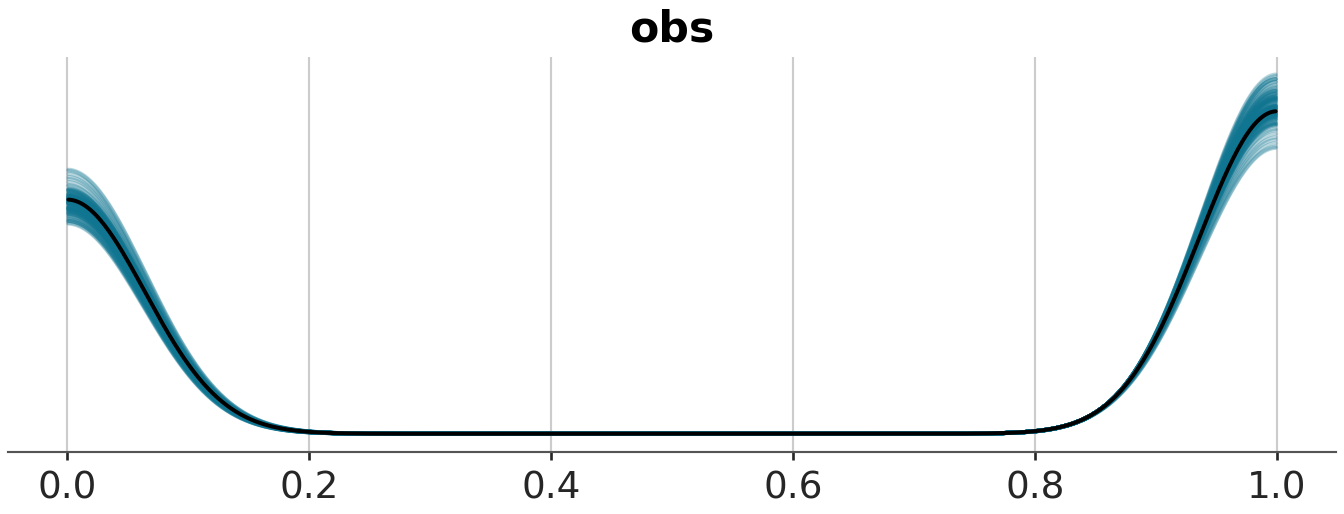
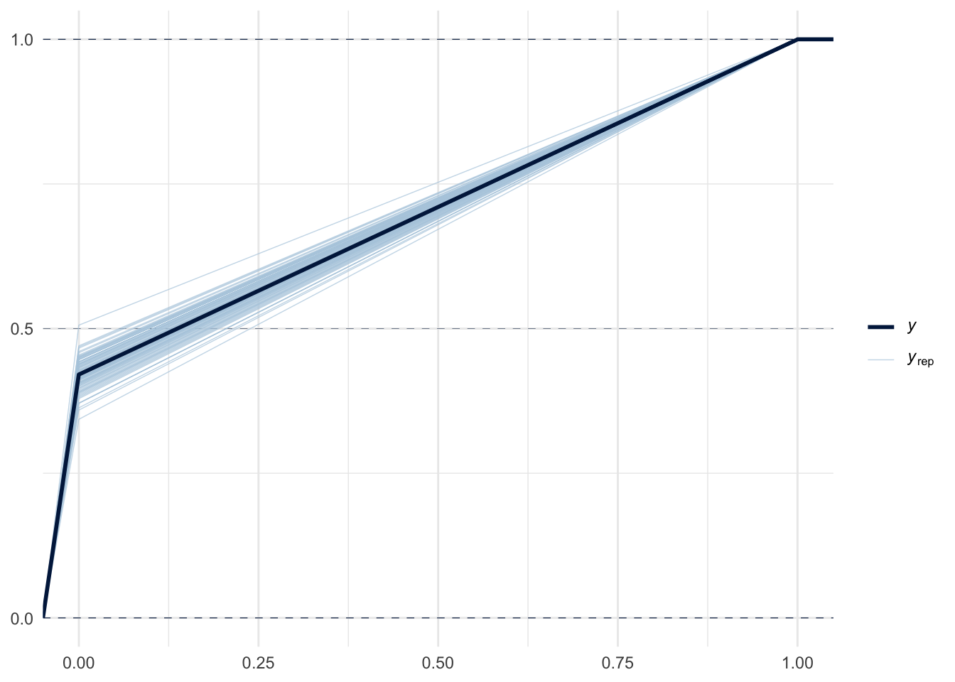
pp_check(m1_prior, ndraws=100, type="dens_overlay")
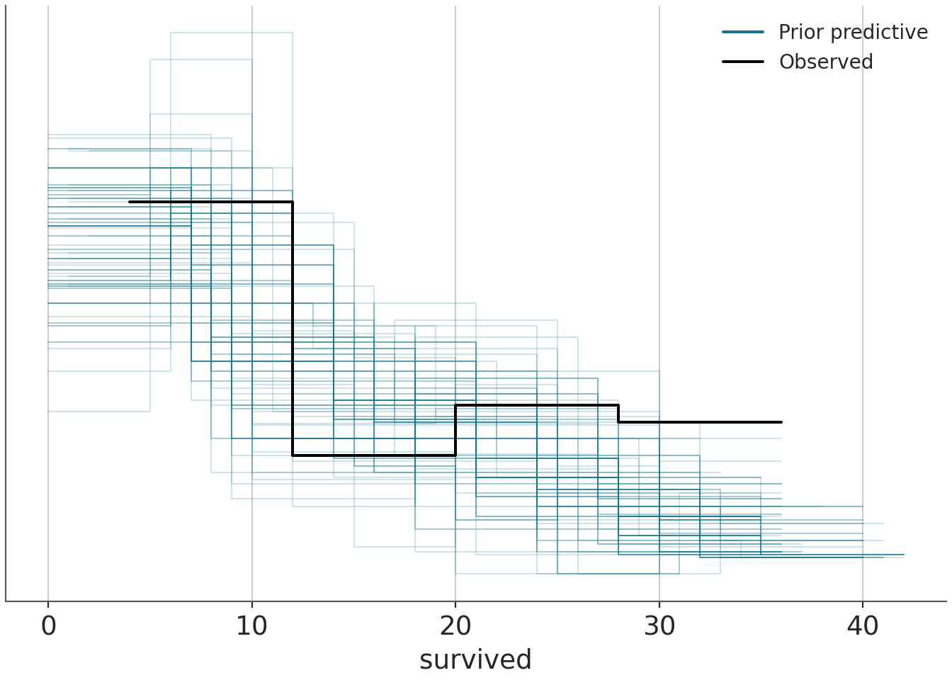
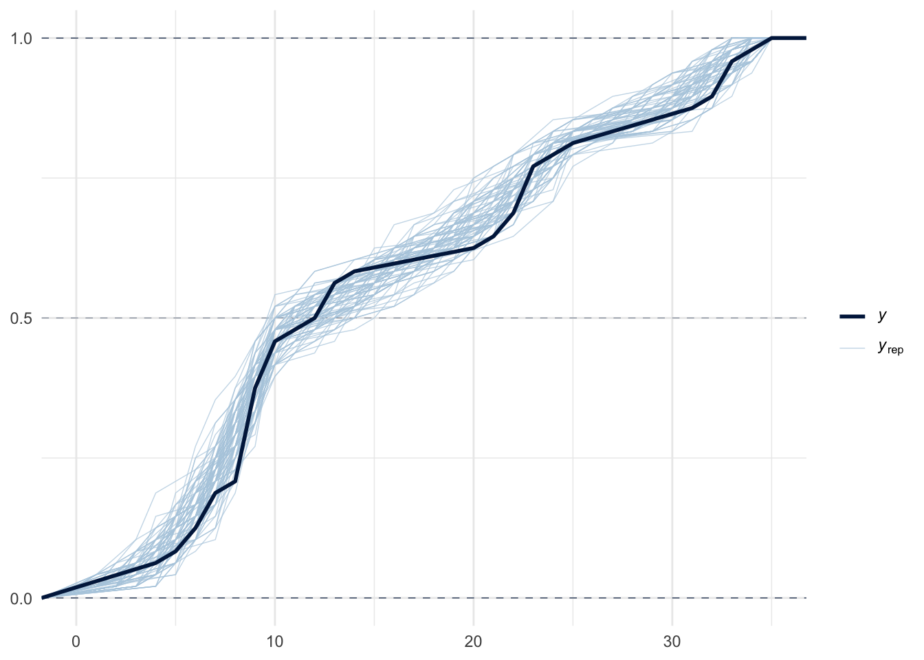
pp_check(m1_prior, ndraws=100, type="ecdf_overlay")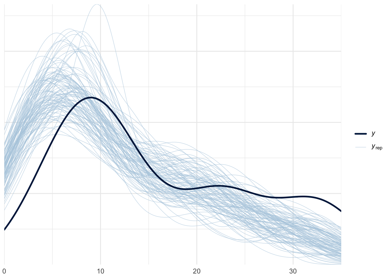

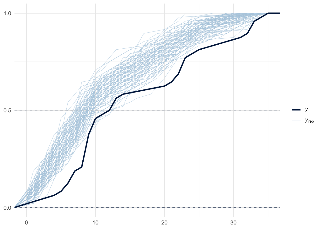
In the above graphs, \(y\) stands for observed data, while \(y_{rep}\) stands for replicated data. The default type for pp_check in bayesplot is dens_overlay, which uses KDE to smooth the data (i.e., probability density for \(y\)) into a continuous curve. ecdf_overlay refers to the empirical cumulative distribution function. We can use these to check whether the prior is “in the ballpark” of the domain knowledge before the actual model fitting. For more on when certain visualization types are appropriate for visual predictive checks in Bayesian workflow, see this paper for more details.

Python

# define the model 
with pm.Model() as model_1:
    # prior 
    alpha = pm.Normal("alpha", 0, 1.5, shape = len(df))
    # link 
    p_survived = pm.Deterministic("p_survived", pm.math.invlogit(alpha))
    # likelihood 
    survived = pm.Binomial("survived", n=df.density, p=p_survived, observed=df.surv)

prior_idata = pm.sample_prior_predictive(model=model_1, draws=100, random_seed=51)
prior_idata

arviz.InferenceData

• prior

  <xarray.Dataset> Size: 78kB
  Dimensions:           (chain: 1, draw: 100, alpha_dim_0: 48,
                         p_survived_dim_0: 48)
  Coordinates:
    * chain             (chain) int64 8B 0
    * draw              (draw) int64 800B 0 1 2 3 4 5 6 7 ... 93 94 95 96 97 98 99
    * alpha_dim_0       (alpha_dim_0) int64 384B 0 1 2 3 4 5 ... 42 43 44 45 46 47
    * p_survived_dim_0  (p_survived_dim_0) int64 384B 0 1 2 3 4 ... 43 44 45 46 47
  Data variables:
      alpha             (chain, draw, alpha_dim_0) float64 38kB -1.175 ... 2.189
      p_survived        (chain, draw, p_survived_dim_0) float64 38kB 0.2359 ......
  Attributes:
      created_at:                 2026-01-25T04:55:29.013021+00:00
      arviz_version:              0.22.0
      inference_library:          pymc
      inference_library_version:  5.26.1

  xarray.Dataset

  • Dimensions:
    • chain: 1
    • draw: 100
    • alpha_dim_0: 48
    • p_survived_dim_0: 48
  • Coordinates: (4)
    • chain
      (chain)
      int64
      0

      array([0])

    • draw
      (draw)
      int64
      0 1 2 3 4 5 6 ... 94 95 96 97 98 99

      array([ 0,  1,  2,  3,  4,  5,  6,  7,  8,  9, 10, 11, 12, 13, 14, 15, 16, 17,
             18, 19, 20, 21, 22, 23, 24, 25, 26, 27, 28, 29, 30, 31, 32, 33, 34, 35,
             36, 37, 38, 39, 40, 41, 42, 43, 44, 45, 46, 47, 48, 49, 50, 51, 52, 53,
             54, 55, 56, 57, 58, 59, 60, 61, 62, 63, 64, 65, 66, 67, 68, 69, 70, 71,
             72, 73, 74, 75, 76, 77, 78, 79, 80, 81, 82, 83, 84, 85, 86, 87, 88, 89,
             90, 91, 92, 93, 94, 95, 96, 97, 98, 99])

    • alpha_dim_0
      (alpha_dim_0)
      int64
      0 1 2 3 4 5 6 ... 42 43 44 45 46 47

      array([ 0,  1,  2,  3,  4,  5,  6,  7,  8,  9, 10, 11, 12, 13, 14, 15, 16, 17,
             18, 19, 20, 21, 22, 23, 24, 25, 26, 27, 28, 29, 30, 31, 32, 33, 34, 35,
             36, 37, 38, 39, 40, 41, 42, 43, 44, 45, 46, 47])

    • p_survived_dim_0
      (p_survived_dim_0)
      int64
      0 1 2 3 4 5 6 ... 42 43 44 45 46 47

      array([ 0,  1,  2,  3,  4,  5,  6,  7,  8,  9, 10, 11, 12, 13, 14, 15, 16, 17,
             18, 19, 20, 21, 22, 23, 24, 25, 26, 27, 28, 29, 30, 31, 32, 33, 34, 35,
             36, 37, 38, 39, 40, 41, 42, 43, 44, 45, 46, 47])

  • Data variables: (2)
    • alpha
      (chain, draw, alpha_dim_0)
      float64
      -1.175 -2.302 ... -0.6341 2.189

      array([[[-1.17541047, -2.30175397, -1.23944767, ...,  1.01571499,
                0.46489656,  1.05094486],
              [-0.12268964, -1.07842545, -0.64443219, ...,  3.22923751,
                0.74942025, -0.34904701],
              [ 2.05358146, -1.17936717, -0.4562528 , ..., -0.57188926,
                1.19932074, -2.59646721],
              ...,
              [ 0.63755181,  4.17257652, -1.64069782, ..., -0.42617744,
               -1.49465727,  0.78196806],
              [-2.13737673, -1.48169223, -2.4653767 , ..., -1.7338376 ,
               -2.64196267, -0.71214081],
              [-1.07112653,  1.21954933,  0.94244575, ...,  0.4315294 ,
               -0.63405821,  2.18866518]]], shape=(1, 100, 48))

    • p_survived
      (chain, draw, p_survived_dim_0)
      float64
      0.2359 0.09098 ... 0.3466 0.8992

      array([[[0.23587841, 0.0909778 , 0.22453214, ..., 0.73413709,
               0.61417513, 0.7409563 ],
              [0.46936601, 0.2538041 , 0.34424533, ..., 0.96191983,
               0.67905236, 0.41361354],
              [0.88630901, 0.235166  , 0.38787514, ..., 0.360801  ,
               0.76840393, 0.06936613],
              ...,
              [0.65419983, 0.98482144, 0.16237013, ..., 0.39503949,
               0.18322372, 0.68610412],
              [0.10551672, 0.18517195, 0.07832133, ..., 0.15009737,
               0.06648612, 0.32912597],
              [0.25518891, 0.77198423, 0.71959342, ..., 0.60623882,
               0.34659092, 0.89922701]]], shape=(1, 100, 48))

  • Attributes: (4)

    created_at :

    2026-01-25T04:55:29.013021+00:00

    arviz_version :

    0.22.0

    inference_library :

    pymc

    inference_library_version :

    5.26.1

  
  
• prior_predictive

  <xarray.Dataset> Size: 40kB
  Dimensions:         (chain: 1, draw: 100, survived_dim_0: 48)
  Coordinates:
    * chain           (chain) int64 8B 0
    * draw            (draw) int64 800B 0 1 2 3 4 5 6 7 ... 93 94 95 96 97 98 99
    * survived_dim_0  (survived_dim_0) int64 384B 0 1 2 3 4 5 ... 43 44 45 46 47
  Data variables:
      survived        (chain, draw, survived_dim_0) int64 38kB 3 1 2 ... 16 12 33
  Attributes:
      created_at:                 2026-01-25T04:55:29.014008+00:00
      arviz_version:              0.22.0
      inference_library:          pymc
      inference_library_version:  5.26.1

  xarray.Dataset

  • Dimensions:
    • chain: 1
    • draw: 100
    • survived_dim_0: 48
  • Coordinates: (3)
    • chain
      (chain)
      int64
      0

      array([0])

    • draw
      (draw)
      int64
      0 1 2 3 4 5 6 ... 94 95 96 97 98 99

      array([ 0,  1,  2,  3,  4,  5,  6,  7,  8,  9, 10, 11, 12, 13, 14, 15, 16, 17,
             18, 19, 20, 21, 22, 23, 24, 25, 26, 27, 28, 29, 30, 31, 32, 33, 34, 35,
             36, 37, 38, 39, 40, 41, 42, 43, 44, 45, 46, 47, 48, 49, 50, 51, 52, 53,
             54, 55, 56, 57, 58, 59, 60, 61, 62, 63, 64, 65, 66, 67, 68, 69, 70, 71,
             72, 73, 74, 75, 76, 77, 78, 79, 80, 81, 82, 83, 84, 85, 86, 87, 88, 89,
             90, 91, 92, 93, 94, 95, 96, 97, 98, 99])

    • survived_dim_0
      (survived_dim_0)
      int64
      0 1 2 3 4 5 6 ... 42 43 44 45 46 47

      array([ 0,  1,  2,  3,  4,  5,  6,  7,  8,  9, 10, 11, 12, 13, 14, 15, 16, 17,
             18, 19, 20, 21, 22, 23, 24, 25, 26, 27, 28, 29, 30, 31, 32, 33, 34, 35,
             36, 37, 38, 39, 40, 41, 42, 43, 44, 45, 46, 47])

  • Data variables: (1)
    • survived
      (chain, draw, survived_dim_0)
      int64
      3 1 2 1 2 0 8 ... 30 2 11 16 12 33

      array([[[ 3,  1,  2, ..., 23, 22, 26],
              [ 3,  1,  4, ..., 34, 22, 13],
              [10,  1,  5, ..., 13, 24,  3],
              ...,
              [ 8, 10,  2, ..., 15,  5, 25],
              [ 1,  2,  1, ...,  3,  5, 10],
              [ 1,  7,  6, ..., 16, 12, 33]]], shape=(1, 100, 48))

  • Attributes: (4)

    created_at :

    2026-01-25T04:55:29.014008+00:00

    arviz_version :

    0.22.0

    inference_library :

    pymc

    inference_library_version :

    5.26.1

  
  
• observed_data

  <xarray.Dataset> Size: 768B
  Dimensions:         (survived_dim_0: 48)
  Coordinates:
    * survived_dim_0  (survived_dim_0) int64 384B 0 1 2 3 4 5 ... 43 44 45 46 47
  Data variables:
      survived        (survived_dim_0) int64 384B 9 10 7 10 9 9 ... 14 22 12 31 17
  Attributes:
      created_at:                 2026-01-25T04:55:29.014418+00:00
      arviz_version:              0.22.0
      inference_library:          pymc
      inference_library_version:  5.26.1

  xarray.Dataset

  • Dimensions:
    • survived_dim_0: 48
  • Coordinates: (1)
    • survived_dim_0
      (survived_dim_0)
      int64
      0 1 2 3 4 5 6 ... 42 43 44 45 46 47

      array([ 0,  1,  2,  3,  4,  5,  6,  7,  8,  9, 10, 11, 12, 13, 14, 15, 16, 17,
             18, 19, 20, 21, 22, 23, 24, 25, 26, 27, 28, 29, 30, 31, 32, 33, 34, 35,
             36, 37, 38, 39, 40, 41, 42, 43, 44, 45, 46, 47])

  • Data variables: (1)
    • survived
      (survived_dim_0)
      int64
      9 10 7 10 9 9 ... 13 14 22 12 31 17

      array([ 9, 10,  7, 10,  9,  9, 10,  9,  4,  9,  7,  6,  7,  5,  9,  9, 24,
             23, 22, 25, 23, 23, 23, 21,  6, 13,  4,  9, 13, 20,  8, 10, 34, 33,
             33, 31, 31, 35, 33, 32,  4, 12, 13, 14, 22, 12, 31, 17])

  • Attributes: (4)

    created_at :

    2026-01-25T04:55:29.014418+00:00

    arviz_version :

    0.22.0

    inference_library :

    pymc

    inference_library_version :

    5.26.1

  
  

az.plot_ppc(prior_idata, group="prior", num_pp_samples=100, observed=True, kind="kde", random_seed=51, mean=False)
azp.plot_ppc_dist(prior_idata, group="prior_predictive", num_samples=100)
azp.plot_ppc_rootogram(prior_idata, group="prior_predictive")

<arviz_plots.plot_collection.PlotCollection object at 0x165da46e0>

<arviz_plots.plot_collection.PlotCollection object at 0x165eb7c50>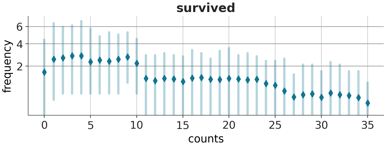

The first plot, plotted using az.plot_ppc is a bit problematic, as it does not appear smoothed as most KDE plots should be.

The second plot, plotted using az.plot_ppc_dist will raise a user warning that it “detects at least one discrete variable” and would then proceed to suggest us to plot using a variant specific for discrete data. There is no option to pass in “observed” to highlight the observed data.

The third plot, plotted using az.plot_ppc_rootogram does not raise any errors.

We could turn the data into more tidy format:

prior_idata.to_dataframe().head(5)

   chain  ...  (prior_predictive, survived[9], 9)
0      0  ...                                   3
1      0  ...                                   5
2      0  ...                                   5
3      0  ...                                   1
4      0  ...                                   5

[5 rows x 146 columns]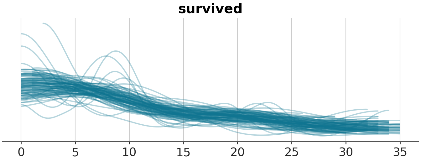

Next step is to fit the actual model²:

² Note that the following corresponds to R code 13.2 in Statistical Rethinking

R

m1 <- brm(formula, 
    family = binomial, data = df, 
    prior = prior(normal(0, 1.5), class = b), 
    cores = parallel::detectCores(), 
    file = here("posts", "pymc-hierarchical", "m1.rds") # prevents re-running the fitting process when quarto compiles  
)

Python

with model_1: 
    model_1_trace = pm.sample(random_seed=51, progressbar=False, nuts_sampler="numpyro")
    model_1_trace = pm.compute_log_likelihood(model_1_trace)
    # posterior predictive check 
    pm.sample_posterior_predictive(model_1_trace, extend_inferencedata=True, random_seed=51)

arviz.InferenceData

• posterior

  <xarray.Dataset> Size: 3MB
  Dimensions:           (chain: 4, draw: 1000, alpha_dim_0: 48,
                         p_survived_dim_0: 48)
  Coordinates:
    * chain             (chain) int64 32B 0 1 2 3
    * draw              (draw) int64 8kB 0 1 2 3 4 5 6 ... 994 995 996 997 998 999
    * alpha_dim_0       (alpha_dim_0) int64 384B 0 1 2 3 4 5 ... 42 43 44 45 46 47
    * p_survived_dim_0  (p_survived_dim_0) int64 384B 0 1 2 3 4 ... 43 44 45 46 47
  Data variables:
      alpha             (chain, draw, alpha_dim_0) float64 2MB 3.214 ... -0.4144
      p_survived        (chain, draw, p_survived_dim_0) float64 2MB 0.9614 ... ...
  Attributes:
      created_at:                 2026-01-25T04:55:33.338147+00:00
      arviz_version:              0.22.0
      inference_library:          numpyro
      inference_library_version:  0.19.0
      sampling_time:              0.628098
      tuning_steps:               1000

  xarray.Dataset

  • Dimensions:
    • chain: 4
    • draw: 1000
    • alpha_dim_0: 48
    • p_survived_dim_0: 48
  • Coordinates: (4)
    • chain
      (chain)
      int64
      0 1 2 3

      array([0, 1, 2, 3])

    • draw
      (draw)
      int64
      0 1 2 3 4 5 ... 995 996 997 998 999

      array([  0,   1,   2, ..., 997, 998, 999], shape=(1000,))

    • alpha_dim_0
      (alpha_dim_0)
      int64
      0 1 2 3 4 5 6 ... 42 43 44 45 46 47

      array([ 0,  1,  2,  3,  4,  5,  6,  7,  8,  9, 10, 11, 12, 13, 14, 15, 16, 17,
             18, 19, 20, 21, 22, 23, 24, 25, 26, 27, 28, 29, 30, 31, 32, 33, 34, 35,
             36, 37, 38, 39, 40, 41, 42, 43, 44, 45, 46, 47])

    • p_survived_dim_0
      (p_survived_dim_0)
      int64
      0 1 2 3 4 5 6 ... 42 43 44 45 46 47

      array([ 0,  1,  2,  3,  4,  5,  6,  7,  8,  9, 10, 11, 12, 13, 14, 15, 16, 17,
             18, 19, 20, 21, 22, 23, 24, 25, 26, 27, 28, 29, 30, 31, 32, 33, 34, 35,
             36, 37, 38, 39, 40, 41, 42, 43, 44, 45, 46, 47])

  • Data variables: (2)
    • alpha
      (chain, draw, alpha_dim_0)
      float64
      3.214 4.324 1.14 ... 1.22 -0.4144

      array([[[ 3.21413748e+00,  4.32386115e+00,  1.13978044e+00, ...,
               -5.86604635e-01,  2.22205560e+00,  2.78209934e-01],
              [ 1.93714607e+00,  2.90786267e+00,  2.29150874e+00, ...,
               -5.73533901e-01,  2.91105088e+00,  1.38954576e-01],
              [ 1.45319770e+00,  2.47898083e+00,  2.10374214e+00, ...,
               -3.63143988e-01,  2.78143080e+00,  1.01617328e-01],
              ...,
              [ 5.61067864e-01,  1.67328399e+00,  1.05053766e+00, ...,
               -3.62260782e-01,  1.42577407e+00,  2.32138785e-02],
              [ 2.50958085e+00,  3.13818420e+00,  1.98146180e-01, ...,
               -7.56960466e-01,  1.96790479e+00,  7.10454035e-02],
              [ 5.01509444e-01,  2.16369741e+00,  2.14642261e+00, ...,
               -3.98560045e-01,  1.74685918e+00,  2.93230431e-02]],
      
             [[ 1.58178129e+00,  3.16858784e+00,  1.69026240e+00, ...,
               -7.25646296e-01,  2.35988897e+00,  8.40907875e-01],
              [ 1.15175818e+00,  1.04987943e+00,  4.12522085e-01, ...,
               -1.15196262e+00,  1.19427777e+00, -1.24668763e-01],
              [ 1.93224806e+00,  4.18451705e+00,  1.04873776e+00, ...,
               -6.96405567e-01,  2.31106211e+00, -2.37805401e-01],
      ...
               -4.66383210e-01,  1.86686841e+00,  3.88370997e-02],
              [ 3.19447766e+00,  2.21703949e+00,  3.87080710e-01, ...,
               -1.00336226e+00,  1.73823594e+00, -1.96658553e-01],
              [ 3.49064036e-01,  3.09012084e+00,  1.18888943e+00, ...,
               -4.33260046e-01,  1.73701328e+00,  3.41918443e-03]],
      
             [[ 8.77544558e-01,  2.14531258e+00,  5.31724908e-01, ...,
               -4.05250536e-01,  2.36398073e+00,  1.04865639e-02],
              [ 1.02001258e+00,  1.19823361e+00,  9.03381253e-01, ...,
               -9.40098840e-01,  1.62003603e+00,  3.71953519e-03],
              [ 1.11590820e+00,  1.63256727e+00,  1.79278948e-01, ...,
               -8.84648344e-01,  2.24534708e+00, -5.90842237e-02],
              ...,
              [ 1.71890354e+00,  2.29953896e+00,  1.43254456e+00, ...,
               -1.12929468e+00,  2.48394264e+00,  1.86806727e-01],
              [ 1.02141999e+00,  2.47751981e+00, -7.97448684e-02, ...,
               -5.22931160e-01,  1.26771631e+00, -1.35056663e-01],
              [ 1.70129521e+00,  2.06628104e+00,  1.08057168e+00, ...,
               -6.87889791e-01,  1.22049516e+00, -4.14413906e-01]]],
            shape=(4, 1000, 48))

    • p_survived
      (chain, draw, p_survived_dim_0)
      float64
      0.9614 0.9869 ... 0.7722 0.3979

      array([[[0.96136284, 0.9869246 , 0.75763933, ..., 0.35741429,
               0.9022127 , 0.56910731],
              [0.87403827, 0.94823375, 0.90817135, ..., 0.3604218 ,
               0.94839003, 0.53468286],
              [0.81049008, 0.9226551 , 0.89126636, ..., 0.41019871,
               0.94166409, 0.52538249],
              ...,
              [0.63669959, 0.84201317, 0.74087813, ..., 0.4104124 ,
               0.80624201, 0.50580321],
              [0.92481075, 0.95844061, 0.5493751 , ..., 0.31930655,
               0.87738589, 0.51775388],
              [0.62281399, 0.89694183, 0.89533401, ..., 0.40165835,
               0.85155621, 0.50733024]],
      
             [[0.82945664, 0.95963492, 0.84425867, ..., 0.32615084,
               0.91371705, 0.69865639],
              [0.75983191, 0.74075175, 0.60169247, ..., 0.24013078,
               0.76750527, 0.46887311],
              [0.87349804, 0.9849989 , 0.74053244, ..., 0.33260964,
               0.90978906, 0.44082725],
      ...
              [0.59324187, 0.91039039, 0.6539256 , ..., 0.38547265,
               0.86609551, 0.50970805],
              [0.96062593, 0.90176926, 0.59557974, ..., 0.26828088,
               0.85046286, 0.4509932 ],
              [0.58639059, 0.9564834 , 0.76654238, ..., 0.39334813,
               0.8503073 , 0.5008548 ]],
      
             [[0.70631313, 0.89522994, 0.62988533, ..., 0.4000515 ,
               0.91403909, 0.50262162],
              [0.73497505, 0.7682104 , 0.71164386, ..., 0.28088038,
               0.8348001 , 0.50092988],
              [0.75322894, 0.83652103, 0.54470008, ..., 0.29221545,
               0.90424843, 0.48523324],
              ...,
              [0.84798755, 0.90883885, 0.80729748, ..., 0.24429129,
               0.92300845, 0.54656634],
              [0.7352491 , 0.92255077, 0.48007434, ..., 0.37216709,
               0.78035157, 0.46628706],
              [0.84570382, 0.88758242, 0.74660215, ..., 0.33450266,
               0.77215068, 0.39785422]]], shape=(4, 1000, 48))

  • Attributes: (6)

    created_at :

    2026-01-25T04:55:33.338147+00:00

    arviz_version :

    0.22.0

    inference_library :

    numpyro

    inference_library_version :

    0.19.0

    sampling_time :

    0.628098

    tuning_steps :

    1000

  
  
• posterior_predictive

  <xarray.Dataset> Size: 2MB
  Dimensions:         (chain: 4, draw: 1000, survived_dim_0: 48)
  Coordinates:
    * chain           (chain) int64 32B 0 1 2 3
    * draw            (draw) int64 8kB 0 1 2 3 4 5 6 ... 994 995 996 997 998 999
    * survived_dim_0  (survived_dim_0) int64 384B 0 1 2 3 4 5 ... 43 44 45 46 47
  Data variables:
      survived        (chain, draw, survived_dim_0) int64 2MB 10 10 8 ... 9 32 12
  Attributes:
      created_at:                 2026-01-25T04:55:36.398150+00:00
      arviz_version:              0.22.0
      inference_library:          pymc
      inference_library_version:  5.26.1

  xarray.Dataset

  • Dimensions:
    • chain: 4
    • draw: 1000
    • survived_dim_0: 48
  • Coordinates: (3)
    • chain
      (chain)
      int64
      0 1 2 3

      array([0, 1, 2, 3])

    • draw
      (draw)
      int64
      0 1 2 3 4 5 ... 995 996 997 998 999

      array([  0,   1,   2, ..., 997, 998, 999], shape=(1000,))

    • survived_dim_0
      (survived_dim_0)
      int64
      0 1 2 3 4 5 6 ... 42 43 44 45 46 47

      array([ 0,  1,  2,  3,  4,  5,  6,  7,  8,  9, 10, 11, 12, 13, 14, 15, 16, 17,
             18, 19, 20, 21, 22, 23, 24, 25, 26, 27, 28, 29, 30, 31, 32, 33, 34, 35,
             36, 37, 38, 39, 40, 41, 42, 43, 44, 45, 46, 47])

  • Data variables: (1)
    • survived
      (chain, draw, survived_dim_0)
      int64
      10 10 8 10 10 10 ... 17 24 9 32 12

      array([[[10, 10,  8, ..., 12, 33, 19],
              [ 7, 10,  9, ..., 14, 35, 22],
              [ 6,  9,  9, ..., 15, 33, 13],
              ...,
              [ 8,  9,  8, ..., 13, 26, 16],
              [10,  8,  8, ..., 12, 30, 20],
              [ 6, 10, 10, ..., 14, 31, 16]],
      
             [[ 8,  9, 10, ..., 15, 33, 28],
              [ 7,  5,  7, ..., 10, 25, 25],
              [ 9, 10,  6, ..., 13, 33, 17],
              ...,
              [ 9, 10,  8, ..., 16, 30, 18],
              [10,  8,  9, ..., 10, 33, 14],
              [ 6, 10,  9, ..., 12, 29, 16]],
      
             [[ 6,  9,  7, ..., 12, 30, 19],
              [10,  9,  7, ..., 14, 30, 15],
              [ 8, 10,  7, ..., 12, 33, 16],
              ...,
              [ 6, 10,  7, ..., 12, 30, 20],
              [10,  8,  8, ..., 10, 32, 14],
              [ 6, 10,  7, ..., 16, 29, 20]],
      
             [[ 4,  9,  6, ..., 10, 30, 22],
              [ 7,  7,  4, ...,  6, 26, 18],
              [ 5,  9,  7, ..., 14, 31, 15],
              ...,
              [ 9,  9,  6, ...,  8, 32, 16],
              [ 9,  9,  5, ..., 12, 27, 20],
              [ 8, 10,  6, ...,  9, 32, 12]]], shape=(4, 1000, 48))

  • Attributes: (4)

    created_at :

    2026-01-25T04:55:36.398150+00:00

    arviz_version :

    0.22.0

    inference_library :

    pymc

    inference_library_version :

    5.26.1

  
  
• log_likelihood

  <xarray.Dataset> Size: 2MB
  Dimensions:         (chain: 4, draw: 1000, survived_dim_0: 48)
  Coordinates:
    * chain           (chain) int64 32B 0 1 2 3
    * draw            (draw) int64 8kB 0 1 2 3 4 5 6 ... 994 995 996 997 998 999
    * survived_dim_0  (survived_dim_0) int64 384B 0 1 2 3 4 5 ... 43 44 45 46 47
  Data variables:
      survived        (chain, draw, survived_dim_0) float64 2MB -1.306 ... -2.563
  Attributes:
      created_at:                 2026-01-25T04:55:36.350181+00:00
      arviz_version:              0.22.0
      inference_library:          pymc
      inference_library_version:  5.26.1

  xarray.Dataset

  • Dimensions:
    • chain: 4
    • draw: 1000
    • survived_dim_0: 48
  • Coordinates: (3)
    • chain
      (chain)
      int64
      0 1 2 3

      array([0, 1, 2, 3])

    • draw
      (draw)
      int64
      0 1 2 3 4 5 ... 995 996 997 998 999

      array([  0,   1,   2, ..., 997, 998, 999], shape=(1000,))

    • survived_dim_0
      (survived_dim_0)
      int64
      0 1 2 3 4 5 6 ... 42 43 44 45 46 47

      array([ 0,  1,  2,  3,  4,  5,  6,  7,  8,  9, 10, 11, 12, 13, 14, 15, 16, 17,
             18, 19, 20, 21, 22, 23, 24, 25, 26, 27, 28, 29, 30, 31, 32, 33, 34, 35,
             36, 37, 38, 39, 40, 41, 42, 43, 44, 45, 46, 47])

  • Data variables: (1)
    • survived
      (chain, draw, survived_dim_0)
      float64
      -1.306 -0.1316 ... -3.066 -2.563

      array([[[-1.30558611, -0.13161634, -1.40732788, ..., -1.9758974 ,
               -1.62399836, -2.50114121],
              [-0.9808721 , -0.53154235, -3.05025654, ..., -1.98324445,
               -2.63293578, -2.17837793],
              [-1.25177443, -0.80499789, -2.67485414, ..., -2.29437808,
               -2.36355803, -2.12046022],
              ...,
              [-2.77305617, -1.71959623, -1.36331256, ..., -2.29646306,
               -2.37519418, -2.03845888],
              [-0.98865733, -0.42447676, -1.79668501, ..., -2.00375255,
               -1.58401401, -2.08209502],
              [-2.93399811, -1.0876427 , -2.75736044, ..., -2.21620306,
               -1.74568019, -2.04291756]],
      
             [[-1.14904058, -0.4120236 , -1.97625903, ..., -1.98168491,
               -1.73185907, -5.45155287],
              [-1.59575351, -3.00089735, -1.53016257, ..., -2.89257902,
               -3.17256068, -2.03011357],
              [-0.98215693, -0.15114754, -1.3625799 , ..., -1.96788681,
               -1.68733788, -2.1524233 ],
      ...
              [-3.29632926, -0.93881773, -1.36914461, ..., -2.09587725,
               -1.63317848, -2.05051141],
              [-1.29359451, -1.03396599, -1.55595029, ..., -2.43061073,
               -1.75615438, -2.09509446],
              [-3.38417067, -0.4449185 , -1.43782945, ..., -2.14984135,
               -1.75766623, -2.02625511]],
      
             [[-2.05192552, -1.10674676, -1.42985791, ..., -2.20262193,
               -1.73589246, -2.03021876],
              [-1.79661474, -2.6369162 , -1.32442898, ..., -2.27936521,
               -1.93395039, -2.02641467],
              [-1.6471837 , -1.78503624, -1.82554465, ..., -2.1700387 ,
               -1.63828025, -2.01022293],
              ...,
              [-1.06521168, -0.95587485, -1.6507725 , ..., -2.81272542,
               -1.87396368, -2.27034956],
              [-1.7942941 , -0.80612867, -2.31141675, ..., -2.02473069,
               -2.88534271, -2.03670679],
              [-1.07457086, -1.19253896, -1.37645158, ..., -1.9651145 ,
               -3.0662274 , -2.56332926]]], shape=(4, 1000, 48))

  • Attributes: (4)

    created_at :

    2026-01-25T04:55:36.350181+00:00

    arviz_version :

    0.22.0

    inference_library :

    pymc

    inference_library_version :

    5.26.1

  
  
• sample_stats

  <xarray.Dataset> Size: 204kB
  Dimensions:          (chain: 4, draw: 1000)
  Coordinates:
    * chain            (chain) int64 32B 0 1 2 3
    * draw             (draw) int64 8kB 0 1 2 3 4 5 6 ... 994 995 996 997 998 999
  Data variables:
      acceptance_rate  (chain, draw) float64 32kB 1.0 0.6541 ... 0.99 0.6298
      step_size        (chain, draw) float64 32kB 0.5056 0.5056 ... 0.4744 0.4744
      diverging        (chain, draw) bool 4kB False False False ... False False
      energy           (chain, draw) float64 32kB 211.7 221.5 ... 203.2 207.6
      n_steps          (chain, draw) int64 32kB 7 7 7 7 7 7 7 7 ... 7 7 7 7 7 7 7
      tree_depth       (chain, draw) int64 32kB 3 3 3 3 3 3 3 3 ... 3 3 3 3 3 3 3
      lp               (chain, draw) float64 32kB 186.7 197.9 ... 182.4 189.0
  Attributes:
      created_at:     2026-01-25T04:55:33.340240+00:00
      arviz_version:  0.22.0

  xarray.Dataset

  • Dimensions:
    • chain: 4
    • draw: 1000
  • Coordinates: (2)
    • chain
      (chain)
      int64
      0 1 2 3

      array([0, 1, 2, 3])

    • draw
      (draw)
      int64
      0 1 2 3 4 5 ... 995 996 997 998 999

      array([  0,   1,   2, ..., 997, 998, 999], shape=(1000,))

  • Data variables: (7)
    • acceptance_rate
      (chain, draw)
      float64
      1.0 0.6541 0.8935 ... 0.99 0.6298

      array([[1.        , 0.65410257, 0.89348918, ..., 0.79693971, 0.76133631,
              0.89798145],
             [0.93663386, 0.95897149, 0.72128395, ..., 0.95205695, 0.78336609,
              0.92127141],
             [1.        , 0.84371839, 0.83127066, ..., 0.75421   , 0.6989561 ,
              0.99730171],
             [0.88009906, 0.73844677, 0.97569455, ..., 0.86452166, 0.99001594,
              0.62975355]], shape=(4, 1000))

    • step_size
      (chain, draw)
      float64
      0.5056 0.5056 ... 0.4744 0.4744

      array([[0.5055622 , 0.5055622 , 0.5055622 , ..., 0.5055622 , 0.5055622 ,
              0.5055622 ],
             [0.42719771, 0.42719771, 0.42719771, ..., 0.42719771, 0.42719771,
              0.42719771],
             [0.50121044, 0.50121044, 0.50121044, ..., 0.50121044, 0.50121044,
              0.50121044],
             [0.47438063, 0.47438063, 0.47438063, ..., 0.47438063, 0.47438063,
              0.47438063]], shape=(4, 1000))

    • diverging
      (chain, draw)
      bool
      False False False ... False False

      array([[False, False, False, ..., False, False, False],
             [False, False, False, ..., False, False, False],
             [False, False, False, ..., False, False, False],
             [False, False, False, ..., False, False, False]], shape=(4, 1000))

    • energy
      (chain, draw)
      float64
      211.7 221.5 217.8 ... 203.2 207.6

      array([[211.72974802, 221.52574906, 217.84106212, ..., 216.71134452,
              216.15565578, 206.39346329],
             [213.03230606, 206.65551404, 210.90044993, ..., 213.17588413,
              220.11927657, 222.63955696],
             [202.12163576, 204.07525924, 213.97001177, ..., 218.14522153,
              211.2703549 , 216.37861447],
             [209.27968524, 207.34060345, 205.94169533, ..., 207.86251159,
              203.22287487, 207.56457017]], shape=(4, 1000))

    • n_steps
      (chain, draw)
      int64
      7 7 7 7 7 7 7 7 ... 7 7 7 7 7 7 7 7

      array([[ 7,  7,  7, ...,  7,  7,  7],
             [ 7,  7,  7, ...,  7, 31,  7],
             [ 7,  7,  7, ...,  7,  7,  7],
             [ 7,  7,  7, ...,  7,  7,  7]], shape=(4, 1000))

    • tree_depth
      (chain, draw)
      int64
      3 3 3 3 3 3 3 3 ... 3 3 3 3 3 3 3 3

      array([[3, 3, 3, ..., 3, 3, 3],
             [3, 3, 3, ..., 3, 5, 3],
             [3, 3, 3, ..., 3, 3, 3],
             [3, 3, 3, ..., 3, 3, 3]], shape=(4, 1000))

    • lp
      (chain, draw)
      float64
      186.7 197.9 189.2 ... 182.4 189.0

      array([[186.68298873, 197.90652396, 189.19716522, ..., 187.10779797,
              185.14920001, 189.80541494],
             [187.48727195, 183.22392225, 189.29132698, ..., 189.38815808,
              193.73360495, 195.45801775],
             [183.01335744, 188.89424728, 186.41619341, ..., 185.964496  ,
              198.56172959, 187.55589387],
             [181.85776435, 187.89935916, 186.55857232, ..., 184.21863152,
              182.3844286 , 189.04365526]], shape=(4, 1000))

  • Attributes: (2)

    created_at :

    2026-01-25T04:55:33.340240+00:00

    arviz_version :

    0.22.0

  
  
• observed_data

  <xarray.Dataset> Size: 768B
  Dimensions:         (survived_dim_0: 48)
  Coordinates:
    * survived_dim_0  (survived_dim_0) int64 384B 0 1 2 3 4 5 ... 43 44 45 46 47
  Data variables:
      survived        (survived_dim_0) int64 384B 9 10 7 10 9 9 ... 14 22 12 31 17
  Attributes:
      created_at:                 2026-01-25T04:55:33.340717+00:00
      arviz_version:              0.22.0
      inference_library:          numpyro
      inference_library_version:  0.19.0
      sampling_time:              0.628098
      tuning_steps:               1000

  xarray.Dataset

  • Dimensions:
    • survived_dim_0: 48
  • Coordinates: (1)
    • survived_dim_0
      (survived_dim_0)
      int64
      0 1 2 3 4 5 6 ... 42 43 44 45 46 47

      array([ 0,  1,  2,  3,  4,  5,  6,  7,  8,  9, 10, 11, 12, 13, 14, 15, 16, 17,
             18, 19, 20, 21, 22, 23, 24, 25, 26, 27, 28, 29, 30, 31, 32, 33, 34, 35,
             36, 37, 38, 39, 40, 41, 42, 43, 44, 45, 46, 47])

  • Data variables: (1)
    • survived
      (survived_dim_0)
      int64
      9 10 7 10 9 9 ... 13 14 22 12 31 17

      array([ 9, 10,  7, 10,  9,  9, 10,  9,  4,  9,  7,  6,  7,  5,  9,  9, 24,
             23, 22, 25, 23, 23, 23, 21,  6, 13,  4,  9, 13, 20,  8, 10, 34, 33,
             33, 31, 31, 35, 33, 32,  4, 12, 13, 14, 22, 12, 31, 17])

  • Attributes: (6)

    created_at :

    2026-01-25T04:55:33.340717+00:00

    arviz_version :

    0.22.0

    inference_library :

    numpyro

    inference_library_version :

    0.19.0

    sampling_time :

    0.628098

    tuning_steps :

    1000

  
  

We can check the fitted model’s summary statistics:

R

summary(m1)

 Family: binomial 
  Links: mu = logit 
Formula: surv | trials(density) ~ 0 + factor(tank) 
   Data: df (Number of observations: 48) 
  Draws: 4 chains, each with iter = 2000; warmup = 1000; thin = 1;
         total post-warmup draws = 4000

Regression Coefficients:
             Estimate Est.Error l-95% CI u-95% CI Rhat Bulk_ESS Tail_ESS
factortank1      1.71      0.78     0.30     3.38 1.00     4841     2773
factortank2      2.41      0.91     0.81     4.38 1.00     5466     2552
factortank3      0.75      0.64    -0.45     2.01 1.00     6429     2893
factortank4      2.42      0.90     0.80     4.37 1.00     5534     2801
factortank5      1.73      0.76     0.40     3.35 1.00     6133     2798
factortank6      1.72      0.77     0.36     3.34 1.00     5855     2831
factortank7      2.42      0.91     0.84     4.34 1.00     4898     2787
factortank8      1.71      0.79     0.26     3.43 1.00     6583     2902
factortank9     -0.36      0.62    -1.61     0.88 1.00     5810     3174
factortank10     1.70      0.76     0.31     3.31 1.00     5849     3072
factortank11     0.75      0.62    -0.45     2.01 1.00     5113     2680
factortank12     0.37      0.60    -0.82     1.57 1.00     5141     2880
factortank13     0.75      0.64    -0.49     2.07 1.00     5751     3041
factortank14     0.00      0.60    -1.19     1.22 1.00     5740     2880
factortank15     1.71      0.78     0.28     3.35 1.00     5165     2245
factortank16     1.72      0.77     0.31     3.30 1.00     6319     2450
factortank17     2.56      0.69     1.36     4.00 1.00     5755     3144
factortank18     2.13      0.59     1.09     3.40 1.00     5396     2874
factortank19     1.80      0.55     0.80     2.95 1.00     5799     2588
factortank20     3.12      0.81     1.70     4.86 1.00     5290     2642
factortank21     2.12      0.61     1.04     3.44 1.00     5753     2748
factortank22     2.13      0.60     1.04     3.41 1.00     4926     2737
factortank23     2.13      0.59     1.11     3.40 1.00     5311     2911
factortank24     1.54      0.50     0.62     2.58 1.00     6062     2666
factortank25    -1.10      0.44    -1.98    -0.28 1.00     5571     3009
factortank26     0.08      0.39    -0.69     0.84 1.00     5045     2869
factortank27    -1.54      0.50    -2.56    -0.60 1.00     5488     2826
factortank28    -0.55      0.40    -1.36     0.21 1.00     6429     2979
factortank29     0.08      0.40    -0.69     0.85 1.00     6081     2796
factortank30     1.31      0.47     0.44     2.29 1.00     5937     2799
factortank31    -0.73      0.42    -1.54     0.06 1.00     5521     2995
factortank32    -0.39      0.40    -1.19     0.39 1.00     6622     3221
factortank33     2.83      0.65     1.70     4.20 1.00     5594     2751
factortank34     2.46      0.59     1.36     3.72 1.00     6757     2890
factortank35     2.46      0.57     1.44     3.70 1.00     5713     2964
factortank36     1.91      0.50     0.98     2.93 1.00     6101     2918
factortank37     1.91      0.48     1.04     2.90 1.00     5749     3220
factortank38     3.37      0.80     1.98     5.09 1.00     5270     2635
factortank39     2.47      0.58     1.45     3.72 1.00     6428     2991
factortank40     2.17      0.53     1.23     3.28 1.00     4563     2679
factortank41    -1.91      0.49    -2.93    -1.02 1.00     6737     2697
factortank42    -0.63      0.36    -1.35     0.06 1.00     6029     2859
factortank43    -0.51      0.35    -1.21     0.16 1.00     6284     2828
factortank44    -0.39      0.33    -1.04     0.25 1.00     6155     3038
factortank45     0.51      0.35    -0.16     1.23 1.00     5068     2723
factortank46    -0.63      0.35    -1.33     0.05 1.00     6318     2773
factortank47     1.92      0.50     1.02     2.97 1.00     6032     2925
factortank48    -0.06      0.34    -0.72     0.58 1.00     6955     2825

Draws were sampled using sampling(NUTS). For each parameter, Bulk_ESS
and Tail_ESS are effective sample size measures, and Rhat is the potential
scale reduction factor on split chains (at convergence, Rhat = 1).

Python

az.summary(model_1_trace)

                 mean     sd  hdi_3%  ...  ess_bulk  ess_tail  r_hat
alpha[0]        1.695  0.759   0.349  ...    5499.0    2681.0    1.0
alpha[1]        2.410  0.903   0.767  ...    5365.0    2646.0    1.0
alpha[2]        0.760  0.638  -0.446  ...    5838.0    2914.0    1.0
alpha[3]        2.410  0.882   0.865  ...    4956.0    2677.0    1.0
alpha[4]        1.704  0.775   0.293  ...    5890.0    2768.0    1.0
...               ...    ...     ...  ...       ...       ...    ...
p_survived[43]  0.404  0.079   0.258  ...    5575.0    3215.0    1.0
p_survived[44]  0.623  0.077   0.473  ...    5024.0    2826.0    1.0
p_survived[45]  0.350  0.075   0.214  ...    5269.0    2997.0    1.0
p_survived[46]  0.861  0.056   0.761  ...    5321.0    2415.0    1.0
p_survived[47]  0.487  0.080   0.335  ...    5712.0    2993.0    1.0

[96 rows x 9 columns]

We can also plot the posterior distribution as well as the trace plot:

R

plot(m1, variable = variables(m1)[1:5])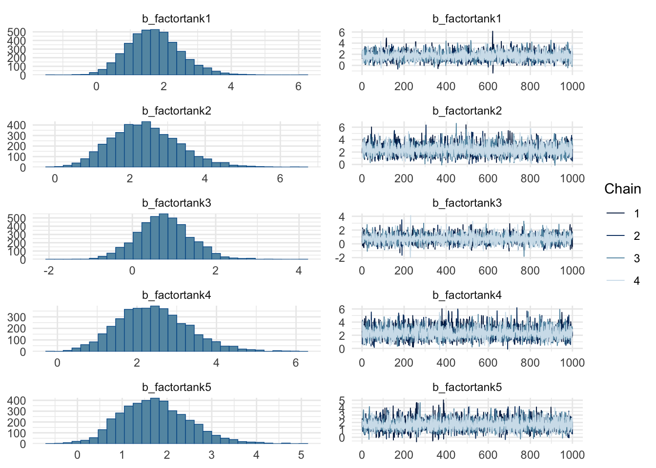

Python

# Pass only the first 5 names to plot_trace
az.plot_trace(model_1_trace, combined=True, var_names="alpha")

array([[<Axes: title={'center': 'alpha'}>,
        <Axes: title={'center': 'alpha'}>]], dtype=object)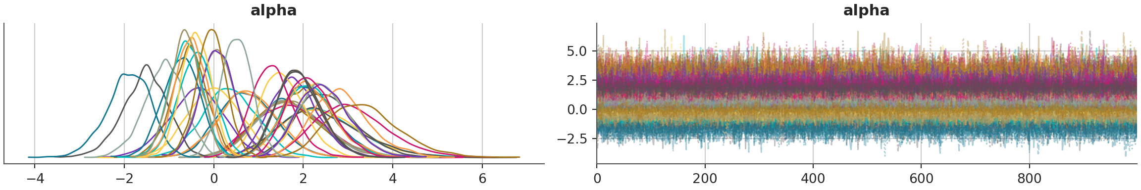

Or something like the “forest plot”:

R

m1 %>% as_draws_df(.) %>% mcmc_intervals(regex_pars = "b_.*")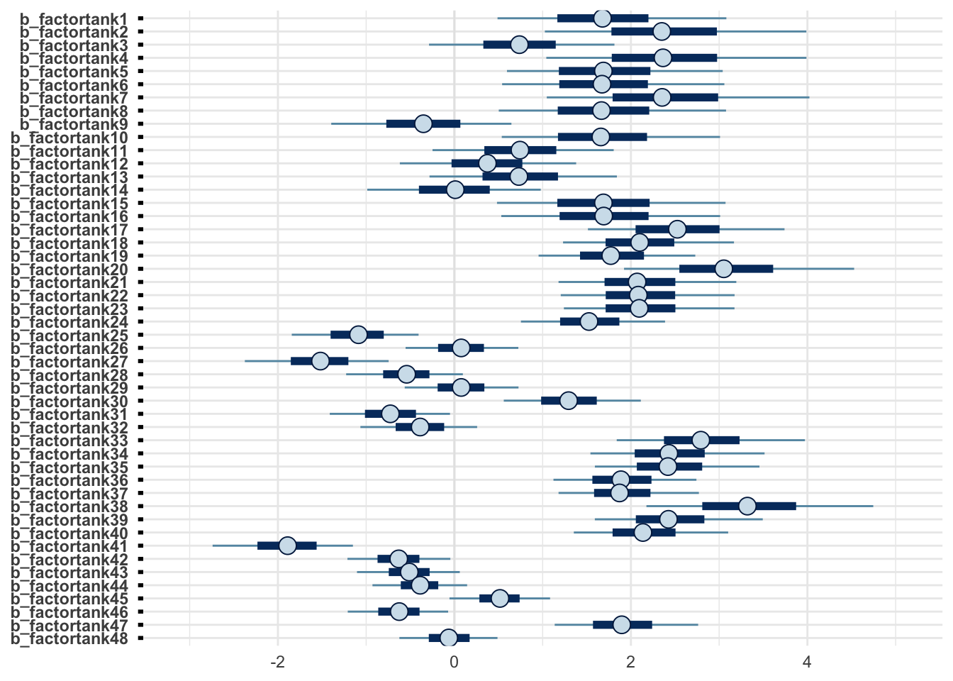

Python

az.plot_forest(model_1_trace, kind='forestplot', combined=True, var_names="alpha", hdi_prob=0.95)

array([<Axes: title={'center': '95.0% HDI'}>], dtype=object)

Note that mcmc_intervals plots the “central (quantile-based) posterior interval estimates from MCMC draws”, while plot_forest displays the credible intervals, where “the central points are the estimated posterior median, the thick lines are the central quantiles, and the thin lines represent the \(100 \times (hdi_prob)\%\) highest density interval”. The former is about equal-tailed intervals (ETI) while the later is about highest density intervals (HDI). The difference between ETI and HDI is negligable between symmetric distribtuions (e.g., Gaussian Normal), but it becomes big when the posterior distributions are skewed. For most common purposes, such as writing about posterior distribtuions in academic journals, most people use ETI because it’s conceptually easier to explain.

We can also perform a posterior predictive check:

R

pp_check(m1, ndraws = 100)
pp_check(m1, ndraws = 100, type="ecdf_overlay")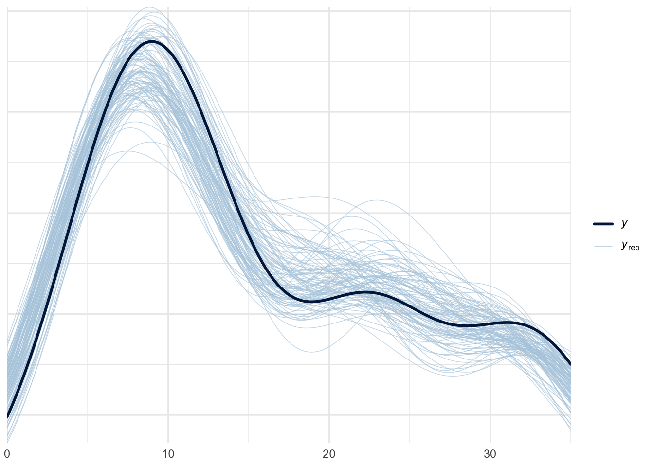

Python

# az.plot_ppc(model_1_trace, num_pp_samples=100)   
azp.plot_ppc_dist(model_1_trace, group="posterior_predictive", num_samples=100)

<arviz_plots.plot_collection.PlotCollection object at 0x42725f4d0>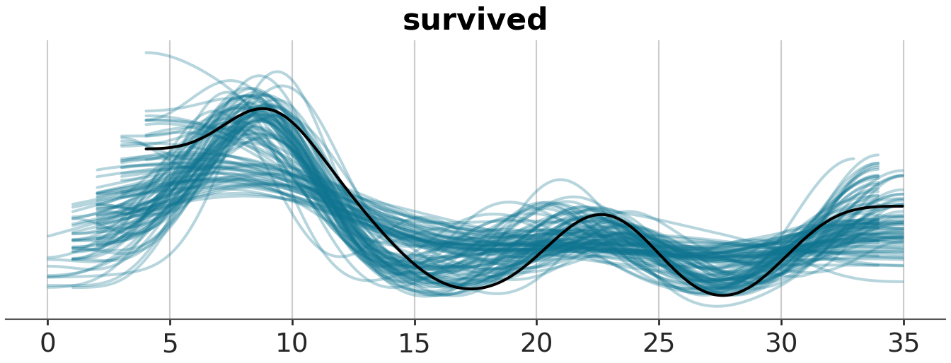

Note on plotting

We can also go beyond the default plots in bayesplot and construct our own plots using ggplot2 and tidybayes. To do that, we first need to get the posterior draws in a tidy format to make it easier for plotting. Observe that the default as_data_frame function does not tell us information related to the chain and draw:

m1 %>% as_tibble(.)

# A tibble: 4,000 × 50
   b_factortank1 b_factortank2 b_factortank3 b_factortank4 b_factortank5
           <dbl>         <dbl>         <dbl>         <dbl>         <dbl>
 1          1.20          1.80        1.77            2.66         2.55 
 2          1.94          2.68       -0.273           1.79         1.38 
 3          1.93          1.97        2.31            2.62         2.15 
 4          2.66          1.71        1.21            1.04         2.24 
 5          2.12          4.06        0.738           3.80         1.15 
 6          1.36          2.74       -0.0728          4.15         1.33 
 7          1.20          3.36       -0.475           1.50         2.59 
 8          2.94          2.08        1.78            1.54         0.891
 9          1.34          2.26       -0.556           3.60         1.69 
10          2.05          3.51        2.08            1.10         1.76 
# ℹ 3,990 more rows
# ℹ 45 more variables: b_factortank6 <dbl>, b_factortank7 <dbl>,
#   b_factortank8 <dbl>, b_factortank9 <dbl>, b_factortank10 <dbl>,
#   b_factortank11 <dbl>, b_factortank12 <dbl>, b_factortank13 <dbl>,
#   b_factortank14 <dbl>, b_factortank15 <dbl>, b_factortank16 <dbl>,
#   b_factortank17 <dbl>, b_factortank18 <dbl>, b_factortank19 <dbl>,
#   b_factortank20 <dbl>, b_factortank21 <dbl>, b_factortank22 <dbl>, …

spread_draws, on the other hand, does provide this information:

m1 %>% spread_draws(`b_factortank.*`, regex = TRUE) %>% 
    # plot the top 5 for now 
    select(1:8) %>% 
    pivot_longer(4:8) %>% 
    ggplot(aes(y = name, x = value)) + 
    stat_halfeye()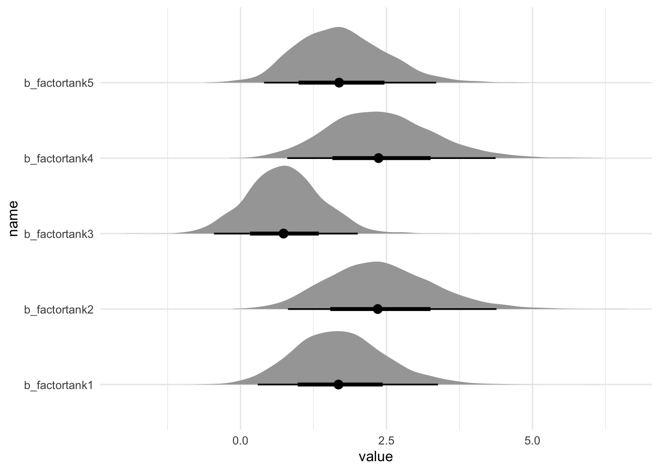

With Pooling

Math model: \[ \begin{align} \texttt{surv}_i &\sim \text{Binomial}(N_i, p_i) \\ \text{logit}(p_i) &\sim \alpha_{\text{TANK}[i]} \\ \alpha_j &\sim \mathcal{N}(\bar{\alpha}, \sigma), j \in [48] \\ \bar{\alpha} &\sim \mathcal{N}(0, 1.5) \\ \sigma &\sim \text{Exponential}(1) \end{align} \]

Here we will skip the prior predictive part and directly go into the model building part³:

³ Note that the following corresponds to R code 13.3 in Statistical Rethinking

R

m2 <- brm(data = df, family = binomial, 
    formula =  bf(surv | trials(density) ~ 1 + (1 | tank)), 
    prior = c(prior(normal(0, 1.5), class = Intercept), 
              prior(exponential(1), class = sd)), 
    cores = parallel::detectCores(), 
    seed = 51, 
    file=here("posts", "pymc-hierarchical", "m2.rds")
)

To get a sense of the default priors that brms gave us:

get_prior(bf(surv | trials(density) ~ 1 + (1 | tank)), family=binomial, data = df)

                prior     class      coef group resp dpar nlpar lb ub tag
 student_t(3, 0, 2.5) Intercept                                          
 student_t(3, 0, 2.5)        sd                                  0       
 student_t(3, 0, 2.5)        sd            tank                  0       
 student_t(3, 0, 2.5)        sd Intercept  tank                  0       
       source
      default
      default
 (vectorized)
 (vectorized)

Python

with pm.Model() as model_2:
    # hyperprior 
    sigma = pm.Exponential("sigma", 1)
    alpha_bar = pm.Normal("alpha_bar", 0, 1.5)
    # prior 
    alpha = pm.Normal("alpha", mu=alpha_bar, sigma=sigma, shape=len(df))
    # link 
    p_survived = pm.Deterministic("p_survived", pm.math.invlogit(alpha))
    # likelihood 
    survived = pm.Binomial("survived", n=df.density, p=p_survived, observed=df.surv)

    model_2_trace = pm.sample(progressbar=False, nuts_sampler="numpyro")
    model_2_trace = pm.compute_log_likelihood(model_2_trace)
    # posterior predictive check 
    pm.sample_posterior_predictive(model_2_trace, extend_inferencedata=True)

arviz.InferenceData

• posterior

  <xarray.Dataset> Size: 3MB
  Dimensions:           (chain: 4, draw: 1000, alpha_dim_0: 48,
                         p_survived_dim_0: 48)
  Coordinates:
    * chain             (chain) int64 32B 0 1 2 3
    * draw              (draw) int64 8kB 0 1 2 3 4 5 6 ... 994 995 996 997 998 999
    * alpha_dim_0       (alpha_dim_0) int64 384B 0 1 2 3 4 5 ... 42 43 44 45 46 47
    * p_survived_dim_0  (p_survived_dim_0) int64 384B 0 1 2 3 4 ... 43 44 45 46 47
  Data variables:
      alpha_bar         (chain, draw) float64 32kB 1.315 1.133 ... 1.485 1.481
      alpha             (chain, draw, alpha_dim_0) float64 2MB 1.898 ... -0.1921
      sigma             (chain, draw) float64 32kB 1.807 1.187 ... 1.668 1.713
      p_survived        (chain, draw, p_survived_dim_0) float64 2MB 0.8696 ... ...
  Attributes:
      created_at:                 2026-01-25T04:55:40.921229+00:00
      arviz_version:              0.22.0
      inference_library:          numpyro
      inference_library_version:  0.19.0
      sampling_time:              0.710105
      tuning_steps:               1000

  xarray.Dataset

  • Dimensions:
    • chain: 4
    • draw: 1000
    • alpha_dim_0: 48
    • p_survived_dim_0: 48
  • Coordinates: (4)
    • chain
      (chain)
      int64
      0 1 2 3

      array([0, 1, 2, 3])

    • draw
      (draw)
      int64
      0 1 2 3 4 5 ... 995 996 997 998 999

      array([  0,   1,   2, ..., 997, 998, 999], shape=(1000,))

    • alpha_dim_0
      (alpha_dim_0)
      int64
      0 1 2 3 4 5 6 ... 42 43 44 45 46 47

      array([ 0,  1,  2,  3,  4,  5,  6,  7,  8,  9, 10, 11, 12, 13, 14, 15, 16, 17,
             18, 19, 20, 21, 22, 23, 24, 25, 26, 27, 28, 29, 30, 31, 32, 33, 34, 35,
             36, 37, 38, 39, 40, 41, 42, 43, 44, 45, 46, 47])

    • p_survived_dim_0
      (p_survived_dim_0)
      int64
      0 1 2 3 4 5 6 ... 42 43 44 45 46 47

      array([ 0,  1,  2,  3,  4,  5,  6,  7,  8,  9, 10, 11, 12, 13, 14, 15, 16, 17,
             18, 19, 20, 21, 22, 23, 24, 25, 26, 27, 28, 29, 30, 31, 32, 33, 34, 35,
             36, 37, 38, 39, 40, 41, 42, 43, 44, 45, 46, 47])

  • Data variables: (4)
    • alpha_bar
      (chain, draw)
      float64
      1.315 1.133 1.294 ... 1.485 1.481

      array([[1.31476129, 1.13267177, 1.29394905, ..., 1.45210912, 1.21190161,
              1.74142008],
             [1.66227389, 1.56519612, 1.42565916, ..., 1.22475236, 1.58564755,
              1.08912212],
             [1.15226983, 1.39907087, 1.17949159, ..., 0.95663462, 1.65892769,
              1.20221817],
             [1.33606084, 1.02608291, 1.99215763, ..., 1.40904046, 1.48504605,
              1.48050631]], shape=(4, 1000))

    • alpha
      (chain, draw, alpha_dim_0)
      float64
      1.898 3.264 ... 2.513 -0.1921

      array([[[ 1.89755042e+00,  3.26350185e+00,  7.01373807e-01, ...,
               -1.07227899e-01,  1.85736403e+00, -3.19894970e-01],
              [ 1.57775808e+00,  1.88208514e+00,  4.60359480e-02, ...,
               -7.40049245e-01,  1.93653270e+00,  2.50326946e-01],
              [ 2.33775171e+00,  4.06737555e+00,  1.81287330e+00, ...,
               -3.53916933e-01,  2.30516507e+00, -2.97726474e-01],
              ...,
              [ 5.90753458e-01,  2.52269671e+00,  1.76273519e+00, ...,
               -1.17115582e-01,  2.02383051e+00, -1.36940786e-01],
              [ 2.28050438e+00,  4.01547750e+00,  1.35278155e+00, ...,
               -1.03941095e+00,  2.27908348e+00,  1.72266598e-01],
              [ 3.89772803e+00,  3.03073691e+00,  9.63919770e-01, ...,
               -1.59581481e-01,  2.22381319e+00, -1.66985300e-01]],
      
             [[ 3.96028858e+00,  3.04841167e+00,  8.27472623e-01, ...,
               -4.63335657e-01,  3.29862621e+00, -5.34604237e-01],
              [ 8.30166280e-01,  2.38311394e+00,  8.99281386e-01, ...,
               -3.27834704e-01,  2.89196167e+00, -5.32896384e-01],
              [ 3.39214350e+00,  3.45683184e+00,  1.62079094e+00, ...,
               -6.31399712e-01,  1.21520824e+00,  2.38272483e-01],
      ...
               -5.87575464e-01,  2.19916701e+00, -5.21234750e-02],
              [ 9.76604247e-01,  3.24999593e+00,  7.01752843e-01, ...,
               -7.54359937e-01,  1.65005575e+00,  5.78377500e-01],
              [ 4.13288771e+00,  2.23617191e+00,  1.28928129e+00, ...,
               -2.76086697e-01,  2.30990798e+00, -4.71403377e-01]],
      
             [[ 1.84434907e+00,  3.21275443e+00,  2.64421843e-01, ...,
               -1.00328584e+00,  2.48522438e+00,  4.25283897e-01],
              [ 2.03182561e+00,  2.27689891e+00,  1.58786615e+00, ...,
               -9.51028077e-02,  1.59499419e+00, -4.11011805e-01],
              [ 2.11121548e+00,  4.50532104e+00,  2.15353999e-01, ...,
               -7.54867410e-01,  2.37948898e+00,  1.12491733e-01],
              ...,
              [ 3.10785569e+00,  3.06439911e+00,  6.49697695e-01, ...,
               -1.05571058e+00,  2.46536440e+00, -1.85826585e-02],
              [ 9.87245554e-01,  2.52526070e+00,  1.06513200e+00, ...,
               -9.32173979e-02,  1.59863604e+00, -6.74026441e-03],
              [ 2.13525373e+00,  1.52390332e+00,  8.64692569e-01, ...,
               -1.46035275e-04,  2.51288252e+00, -1.92130465e-01]]],
            shape=(4, 1000, 48))

    • sigma
      (chain, draw)
      float64
      1.807 1.187 1.353 ... 1.668 1.713

      array([[1.80728447, 1.18712238, 1.35347523, ..., 1.56403119, 2.06759881,
              1.46035192],
             [1.70755915, 1.56192865, 1.71683838, ..., 1.60447617, 1.92692509,
              1.20219869],
             [1.44478674, 1.40110064, 1.93948493, ..., 1.93200448, 1.57111721,
              1.8164648 ],
             [1.30085006, 1.42298135, 2.34568192, ..., 1.63050558, 1.66844086,
              1.71254956]], shape=(4, 1000))

    • p_survived
      (chain, draw, p_survived_dim_0)
      float64
      0.8696 0.9632 ... 0.925 0.4521

      array([[[0.86961403, 0.96315526, 0.66849229, ..., 0.47321868,
               0.86498941, 0.42070134],
              [0.82888677, 0.86785045, 0.51150695, ..., 0.32299338,
               0.87397073, 0.56225697],
              [0.91195573, 0.98316597, 0.85970878, ..., 0.4124329 ,
               0.90930391, 0.42611336],
              ...,
              [0.64353801, 0.92571771, 0.85355189, ..., 0.47075452,
               0.88327651, 0.4658182 ],
              [0.9072495 , 0.98228513, 0.79458401, ..., 0.26126367,
               0.90712986, 0.54296046],
              [0.98011546, 0.95394356, 0.72390592, ..., 0.46018908,
               0.90236765, 0.45835041]],
      
             [[0.98129879, 0.9547139 , 0.69582026, ..., 0.38619481,
               0.96438165, 0.36944366],
              [0.69639009, 0.91553056, 0.7108018 , ..., 0.41876757,
               0.94744764, 0.36984161],
              [0.9674581 , 0.96943423, 0.83490418, ..., 0.34719323,
               0.77121919, 0.55928789],
      ...
              [0.96181738, 0.88179416, 0.78132772, ..., 0.35719135,
               0.90017468, 0.48697208],
              [0.72643391, 0.96267297, 0.66857629, ..., 0.31987204,
               0.83889859, 0.64069398],
              [0.98421661, 0.90345106, 0.78402551, ..., 0.43141343,
               0.9096943 , 0.38428414]],
      
             [[0.86346225, 0.96131144, 0.56572297, ..., 0.26829588,
               0.92309948, 0.60474695],
              [0.88409828, 0.90694566, 0.83031567, ..., 0.4762422 ,
               0.83131759, 0.39866953],
              [0.89198849, 0.98907073, 0.55363139, ..., 0.31976164,
               0.9152498 , 0.52809331],
              ...,
              [0.95721562, 0.95540012, 0.65694234, ..., 0.25813002,
               0.92167778, 0.49535447],
              [0.72854352, 0.92589382, 0.74367006, ..., 0.47671251,
               0.83182767, 0.49831494],
              [0.89428273, 0.82111255, 0.70364013, ..., 0.49996349,
               0.92504001, 0.4521146 ]]], shape=(4, 1000, 48))

  • Attributes: (6)

    created_at :

    2026-01-25T04:55:40.921229+00:00

    arviz_version :

    0.22.0

    inference_library :

    numpyro

    inference_library_version :

    0.19.0

    sampling_time :

    0.710105

    tuning_steps :

    1000

  
  
• posterior_predictive

  <xarray.Dataset> Size: 2MB
  Dimensions:         (chain: 4, draw: 1000, survived_dim_0: 48)
  Coordinates:
    * chain           (chain) int64 32B 0 1 2 3
    * draw            (draw) int64 8kB 0 1 2 3 4 5 6 ... 994 995 996 997 998 999
    * survived_dim_0  (survived_dim_0) int64 384B 0 1 2 3 4 5 ... 43 44 45 46 47
  Data variables:
      survived        (chain, draw, survived_dim_0) int64 2MB 8 10 5 ... 12 33 12
  Attributes:
      created_at:                 2026-01-25T04:55:44.023908+00:00
      arviz_version:              0.22.0
      inference_library:          pymc
      inference_library_version:  5.26.1

  xarray.Dataset

  • Dimensions:
    • chain: 4
    • draw: 1000
    • survived_dim_0: 48
  • Coordinates: (3)
    • chain
      (chain)
      int64
      0 1 2 3

      array([0, 1, 2, 3])

    • draw
      (draw)
      int64
      0 1 2 3 4 5 ... 995 996 997 998 999

      array([  0,   1,   2, ..., 997, 998, 999], shape=(1000,))

    • survived_dim_0
      (survived_dim_0)
      int64
      0 1 2 3 4 5 6 ... 42 43 44 45 46 47

      array([ 0,  1,  2,  3,  4,  5,  6,  7,  8,  9, 10, 11, 12, 13, 14, 15, 16, 17,
             18, 19, 20, 21, 22, 23, 24, 25, 26, 27, 28, 29, 30, 31, 32, 33, 34, 35,
             36, 37, 38, 39, 40, 41, 42, 43, 44, 45, 46, 47])

  • Data variables: (1)
    • survived
      (chain, draw, survived_dim_0)
      int64
      8 10 5 10 9 9 ... 15 10 19 12 33 12

      array([[[ 8, 10,  5, ..., 20, 26, 13],
              [ 7,  8,  6, ..., 14, 29, 13],
              [ 9, 10,  9, ..., 12, 31, 16],
              ...,
              [ 6,  9,  9, ..., 15, 33,  7],
              [ 8, 10,  8, ...,  4, 33, 23],
              [ 9, 10,  6, ..., 18, 33, 14]],
      
             [[10, 10,  5, ..., 11, 34, 11],
              [ 8, 10,  7, ..., 17, 31, 15],
              [10, 10, 10, ..., 14, 27, 18],
              ...,
              [ 9, 10,  8, ...,  6, 32, 20],
              [ 9, 10,  9, ..., 20, 29, 17],
              [ 8,  9,  5, ...,  8, 32, 16]],
      
             [[ 8,  8,  8, ..., 11, 31, 16],
              [ 9, 10,  5, ..., 15, 32, 21],
              [ 9,  9,  8, ...,  7, 28, 17],
              ...,
              [ 7,  9, 10, ..., 10, 28, 15],
              [ 9, 10,  6, ..., 12, 30, 22],
              [10,  8,  9, ...,  8, 30, 13]],
      
             [[ 7, 10,  7, ...,  9, 29, 18],
              [10, 10,  8, ..., 15, 26, 13],
              [10, 10,  5, ..., 15, 31, 18],
              ...,
              [10, 10,  8, ..., 10, 31, 20],
              [ 9,  9,  7, ..., 21, 30, 19],
              [10,  9,  7, ..., 12, 33, 12]]], shape=(4, 1000, 48))

  • Attributes: (4)

    created_at :

    2026-01-25T04:55:44.023908+00:00

    arviz_version :

    0.22.0

    inference_library :

    pymc

    inference_library_version :

    5.26.1

  
  
• log_likelihood

  <xarray.Dataset> Size: 2MB
  Dimensions:         (chain: 4, draw: 1000, survived_dim_0: 48)
  Coordinates:
    * chain           (chain) int64 32B 0 1 2 3
    * draw            (draw) int64 8kB 0 1 2 3 4 5 6 ... 994 995 996 997 998 999
    * survived_dim_0  (survived_dim_0) int64 384B 0 1 2 3 4 5 ... 43 44 45 46 47
  Data variables:
      survived        (chain, draw, survived_dim_0) float64 2MB -0.992 ... -2.09
  Attributes:
      created_at:                 2026-01-25T04:55:43.965596+00:00
      arviz_version:              0.22.0
      inference_library:          pymc
      inference_library_version:  5.26.1

  xarray.Dataset

  • Dimensions:
    • chain: 4
    • draw: 1000
    • survived_dim_0: 48
  • Coordinates: (3)
    • chain
      (chain)
      int64
      0 1 2 3

      array([0, 1, 2, 3])

    • draw
      (draw)
      int64
      0 1 2 3 4 5 ... 995 996 997 998 999

      array([  0,   1,   2, ..., 997, 998, 999], shape=(1000,))

    • survived_dim_0
      (survived_dim_0)
      int64
      0 1 2 3 4 5 6 ... 42 43 44 45 46 47

      array([ 0,  1,  2,  3,  4,  5,  6,  7,  8,  9, 10, 11, 12, 13, 14, 15, 16, 17,
             18, 19, 20, 21, 22, 23, 24, 25, 26, 27, 28, 29, 30, 31, 32, 33, 34, 35,
             36, 37, 38, 39, 40, 41, 42, 43, 44, 45, 46, 47])

  • Data variables: (1)
    • survived
      (chain, draw, survived_dim_0)
      float64
      -0.992 -0.3754 ... -1.913 -2.09

      array([[[-0.99202342, -0.37540651, -1.3439338 , ..., -3.17839123,
               -1.63988849, -2.31035682],
              [-1.15189014, -1.41735875, -2.05455707, ..., -1.99090313,
               -1.59502637, -2.42309818],
              [-0.95680492, -0.16977332, -2.16274391, ..., -2.31648649,
               -1.68241896, -2.26201184],
              ...,
              [-2.6959103 , -0.77185944, -2.08420322, ..., -3.13370358,
               -1.57351803, -2.03800336],
              [-0.95129715, -0.17873651, -1.57021856, ..., -2.52914325,
               -1.66187381, -2.240299  ],
              [-1.79599188, -0.47150771, -1.33520594, ..., -2.95146445,
               -1.62501803, -2.06285315]],
      
             [[-1.84648641, -0.4634356 , -1.32156506, ..., -2.10046132,
               -3.59799217, -2.99296229],
              [-2.14603424, -0.88251534, -1.32396885, ..., -2.38288994,
               -2.59137462, -2.98602412],
              [-1.42039008, -0.31042647, -1.87926421, ..., -1.96110441,
               -3.08732761, -2.39143053],
      ...
              [-1.3131659 , -1.25796627, -1.50037581, ..., -1.97540655,
               -1.61159529, -2.01031754],
              [-1.87009692, -0.38041524, -1.34381453, ..., -2.00163474,
               -1.88261573, -3.75725498],
              [-1.98939539, -1.01533337, -1.51348927, ..., -2.53181457,
               -1.6863673 , -2.75213937]],
      
             [[-1.00981494, -0.39456846, -1.70228158, ..., -2.43041127,
               -1.87563877, -3.02253448],
              [-0.96111101, -0.97672743, -1.83559992, ..., -3.23435531,
               -1.98009677, -2.55291598],
              [-0.95165084, -0.10989436, -1.77113207, ..., -2.00204397,
               -1.75159613, -2.13607403],
              ...,
              [-1.2425366 , -0.4562505 , -1.36319168, ..., -2.57658631,
               -1.85014507, -2.01671378],
              [-1.85173956, -0.76995711, -1.36948243, ..., -3.24317282,
               -1.97319563, -2.021323  ],
              [-0.95000163, -1.97095095, -1.32146824, ..., -3.71706268,
               -1.91277186, -2.08968061]]], shape=(4, 1000, 48))

  • Attributes: (4)

    created_at :

    2026-01-25T04:55:43.965596+00:00

    arviz_version :

    0.22.0

    inference_library :

    pymc

    inference_library_version :

    5.26.1

  
  
• sample_stats

  <xarray.Dataset> Size: 204kB
  Dimensions:          (chain: 4, draw: 1000)
  Coordinates:
    * chain            (chain) int64 32B 0 1 2 3
    * draw             (draw) int64 8kB 0 1 2 3 4 5 6 ... 994 995 996 997 998 999
  Data variables:
      acceptance_rate  (chain, draw) float64 32kB 0.9605 0.9454 ... 0.7808 0.9038
      step_size        (chain, draw) float64 32kB 0.3739 0.3739 ... 0.4353 0.4353
      diverging        (chain, draw) bool 4kB False False False ... False False
      energy           (chain, draw) float64 32kB 203.3 205.2 ... 221.2 215.1
      n_steps          (chain, draw) int64 32kB 15 15 15 15 15 15 ... 7 15 7 7 15
      tree_depth       (chain, draw) int64 32kB 4 4 4 4 4 4 4 4 ... 3 5 3 4 3 3 4
      lp               (chain, draw) float64 32kB 179.5 173.8 ... 184.3 185.3
  Attributes:
      created_at:     2026-01-25T04:55:40.923475+00:00
      arviz_version:  0.22.0

  xarray.Dataset

  • Dimensions:
    • chain: 4
    • draw: 1000
  • Coordinates: (2)
    • chain
      (chain)
      int64
      0 1 2 3

      array([0, 1, 2, 3])

    • draw
      (draw)
      int64
      0 1 2 3 4 5 ... 995 996 997 998 999

      array([  0,   1,   2, ..., 997, 998, 999], shape=(1000,))

  • Data variables: (7)
    • acceptance_rate
      (chain, draw)
      float64
      0.9605 0.9454 ... 0.7808 0.9038

      array([[0.96047937, 0.94540801, 0.77508289, ..., 0.98623018, 0.98715549,
              0.9947451 ],
             [0.93816594, 0.86917149, 0.98806925, ..., 0.92123196, 0.86946669,
              0.97146891],
             [0.88744407, 0.96005821, 0.9663061 , ..., 0.83345648, 0.80600704,
              0.87508686],
             [0.98389418, 0.86571119, 0.77348179, ..., 0.93754863, 0.78080407,
              0.9037787 ]], shape=(4, 1000))

    • step_size
      (chain, draw)
      float64
      0.3739 0.3739 ... 0.4353 0.4353

      array([[0.37391977, 0.37391977, 0.37391977, ..., 0.37391977, 0.37391977,
              0.37391977],
             [0.41349196, 0.41349196, 0.41349196, ..., 0.41349196, 0.41349196,
              0.41349196],
             [0.41569871, 0.41569871, 0.41569871, ..., 0.41569871, 0.41569871,
              0.41569871],
             [0.43525187, 0.43525187, 0.43525187, ..., 0.43525187, 0.43525187,
              0.43525187]], shape=(4, 1000))

    • diverging
      (chain, draw)
      bool
      False False False ... False False

      array([[False, False, False, ..., False, False, False],
             [False, False, False, ..., False, False, False],
             [False, False, False, ..., False, False, False],
             [False, False, False, ..., False, False, False]], shape=(4, 1000))

    • energy
      (chain, draw)
      float64
      203.3 205.2 195.4 ... 221.2 215.1

      array([[203.29816975, 205.19258669, 195.38039632, ..., 210.16117992,
              212.20210082, 209.68688661],
             [199.05197918, 203.56681448, 207.71855608, ..., 210.12445148,
              216.19684273, 211.61349199],
             [199.8692596 , 197.64453121, 193.30856112, ..., 204.42166068,
              218.80699695, 215.66376736],
             [199.95878943, 203.21242265, 204.86529677, ..., 208.84768013,
              221.1743507 , 215.08232202]], shape=(4, 1000))

    • n_steps
      (chain, draw)
      int64
      15 15 15 15 15 15 ... 7 15 7 7 15

      array([[15, 15, 15, ..., 15, 15, 15],
             [15,  7, 15, ..., 15, 15, 15],
             [ 7,  7, 15, ...,  7,  7, 31],
             [ 7,  7,  7, ...,  7,  7, 15]], shape=(4, 1000))

    • tree_depth
      (chain, draw)
      int64
      4 4 4 4 4 4 4 4 ... 3 3 5 3 4 3 3 4

      array([[4, 4, 4, ..., 4, 4, 4],
             [4, 3, 4, ..., 4, 4, 4],
             [3, 3, 4, ..., 3, 3, 5],
             [3, 3, 3, ..., 3, 3, 4]], shape=(4, 1000))

    • lp
      (chain, draw)
      float64
      179.5 173.8 176.8 ... 184.3 185.3

      array([[179.47014363, 173.78156734, 176.81638812, ..., 184.76917213,
              187.90964972, 182.44293315],
             [176.33934714, 184.82186143, 185.6962566 , ..., 185.63492147,
              188.66175005, 190.03487122],
             [175.85400257, 174.84360194, 173.83472296, ..., 183.9528557 ,
              186.93143401, 185.05748619],
             [178.25274405, 175.01239991, 183.38298575, ..., 185.53396342,
              184.29972774, 185.25002414]], shape=(4, 1000))

  • Attributes: (2)

    created_at :

    2026-01-25T04:55:40.923475+00:00

    arviz_version :

    0.22.0

  
  
• observed_data

  <xarray.Dataset> Size: 768B
  Dimensions:         (survived_dim_0: 48)
  Coordinates:
    * survived_dim_0  (survived_dim_0) int64 384B 0 1 2 3 4 5 ... 43 44 45 46 47
  Data variables:
      survived        (survived_dim_0) int64 384B 9 10 7 10 9 9 ... 14 22 12 31 17
  Attributes:
      created_at:                 2026-01-25T04:55:40.923931+00:00
      arviz_version:              0.22.0
      inference_library:          numpyro
      inference_library_version:  0.19.0
      sampling_time:              0.710105
      tuning_steps:               1000

  xarray.Dataset

  • Dimensions:
    • survived_dim_0: 48
  • Coordinates: (1)
    • survived_dim_0
      (survived_dim_0)
      int64
      0 1 2 3 4 5 6 ... 42 43 44 45 46 47

      array([ 0,  1,  2,  3,  4,  5,  6,  7,  8,  9, 10, 11, 12, 13, 14, 15, 16, 17,
             18, 19, 20, 21, 22, 23, 24, 25, 26, 27, 28, 29, 30, 31, 32, 33, 34, 35,
             36, 37, 38, 39, 40, 41, 42, 43, 44, 45, 46, 47])

  • Data variables: (1)
    • survived
      (survived_dim_0)
      int64
      9 10 7 10 9 9 ... 13 14 22 12 31 17

      array([ 9, 10,  7, 10,  9,  9, 10,  9,  4,  9,  7,  6,  7,  5,  9,  9, 24,
             23, 22, 25, 23, 23, 23, 21,  6, 13,  4,  9, 13, 20,  8, 10, 34, 33,
             33, 31, 31, 35, 33, 32,  4, 12, 13, 14, 22, 12, 31, 17])

  • Attributes: (6)

    created_at :

    2026-01-25T04:55:40.923931+00:00

    arviz_version :

    0.22.0

    inference_library :

    numpyro

    inference_library_version :

    0.19.0

    sampling_time :

    0.710105

    tuning_steps :

    1000

  
  

We can check the summary as well as the traces:

R

summary(m2)

 Family: binomial 
  Links: mu = logit 
Formula: surv | trials(density) ~ 1 + (1 | tank) 
   Data: df (Number of observations: 48) 
  Draws: 4 chains, each with iter = 2000; warmup = 1000; thin = 1;
         total post-warmup draws = 4000

Multilevel Hyperparameters:
~tank (Number of levels: 48) 
              Estimate Est.Error l-95% CI u-95% CI Rhat Bulk_ESS Tail_ESS
sd(Intercept)     1.61      0.21     1.25     2.08 1.00      901     1890

Regression Coefficients:
          Estimate Est.Error l-95% CI u-95% CI Rhat Bulk_ESS Tail_ESS
Intercept     1.34      0.26     0.86     1.86 1.00      652     1361

Draws were sampled using sampling(NUTS). For each parameter, Bulk_ESS
and Tail_ESS are effective sample size measures, and Rhat is the potential
scale reduction factor on split chains (at convergence, Rhat = 1).

plot(m2)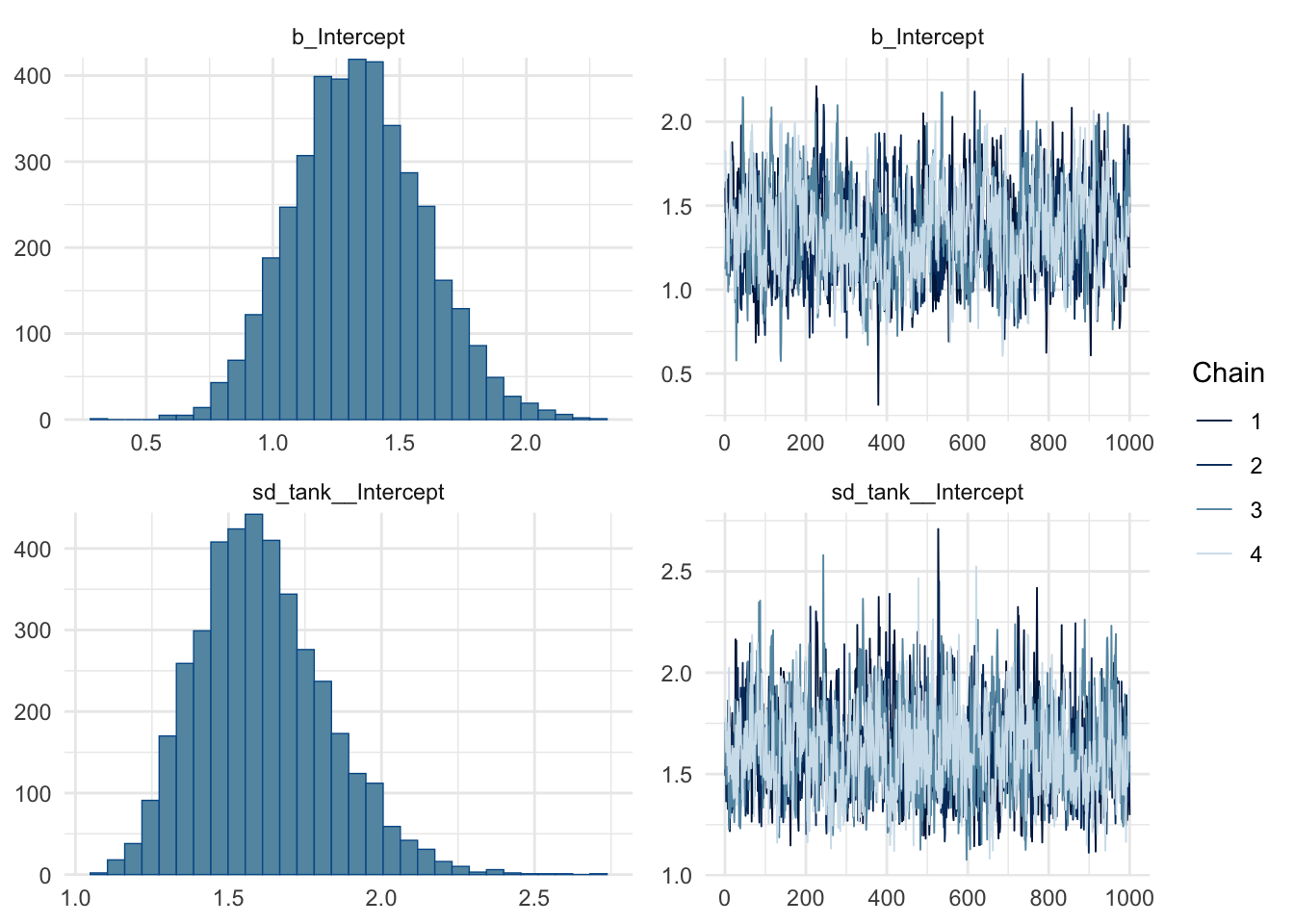

Python

az.summary(model_2_trace)

                 mean     sd  hdi_3%  ...  ess_bulk  ess_tail  r_hat
alpha_bar       1.353  0.261   0.838  ...    4411.0    2731.0    1.0
alpha[0]        2.146  0.876   0.609  ...    5025.0    2354.0    1.0
alpha[1]        3.078  1.083   1.134  ...    4227.0    2324.0    1.0
alpha[2]        1.009  0.650  -0.156  ...    5064.0    2655.0    1.0
alpha[3]        3.100  1.148   1.131  ...    4328.0    2543.0    1.0
...               ...    ...     ...  ...       ...       ...    ...
p_survived[43]  0.420  0.080   0.272  ...    5501.0    3006.0    1.0
p_survived[44]  0.638  0.079   0.491  ...    5555.0    2380.0    1.0
p_survived[45]  0.365  0.079   0.223  ...    5210.0    2807.0    1.0
p_survived[46]  0.877  0.053   0.782  ...    5256.0    3257.0    1.0
p_survived[47]  0.502  0.080   0.356  ...    5217.0    3264.0    1.0

[98 rows x 9 columns]

Model comparison

Now that we have two models for the tadpole dataset, we can compare them using …

R

… the loo package in R:

loo(m1, m2)

Output of model 'm1':

Computed from 4000 by 48 log-likelihood matrix.

         Estimate  SE
elpd_loo   -121.5 2.4
p_loo        39.8 2.0
looic       243.1 4.9
------
MCSE of elpd_loo is NA.
MCSE and ESS estimates assume MCMC draws (r_eff in [0.4, 1.5]).

Pareto k diagnostic values:
                         Count Pct.    Min. ESS
(-Inf, 0.7]   (good)      7    14.6%   182     
   (0.7, 1]   (bad)      34    70.8%   <NA>    
   (1, Inf)   (very bad)  7    14.6%   <NA>    
See help('pareto-k-diagnostic') for details.

Output of model 'm2':

Computed from 4000 by 48 log-likelihood matrix.

         Estimate  SE
elpd_loo   -110.6 4.1
p_loo        31.5 1.5
looic       221.2 8.3
------
MCSE of elpd_loo is NA.
MCSE and ESS estimates assume MCMC draws (r_eff in [0.3, 1.5]).

Pareto k diagnostic values:
                         Count Pct.    Min. ESS
(-Inf, 0.7]   (good)      5    10.4%   194     
   (0.7, 1]   (bad)      40    83.3%   <NA>    
   (1, Inf)   (very bad)  3     6.2%   <NA>    
See help('pareto-k-diagnostic') for details.

Model comparisons:
   elpd_diff se_diff
m2   0.0       0.0  
m1 -10.9       2.8  

Python

az.compare({'unpooled': model_1_trace, 'pooled': model_2_trace})

          rank    elpd_loo      p_loo  ...      dse  warning  scale
pooled       0 -110.475998  31.455554  ...  0.00000     True    log
unpooled     1 -120.078198  38.335198  ...  2.60797     True    log

[2 rows x 9 columns]

Multilevel Chimpanzees

Next we will explore the chimpanzee dataset for something a bit more complex to demonstrate the power of the PyMC syntax. The chimpanzee data is obtained from here. The example we’re looking at is 13.3.1 Multilevel chimpanzees. We will create a new column, treatment, that is a combination of prosoc_left and condition.

Here’s the math model: \[ \begin{align} \texttt{pulled\_left}_i &\sim \text{Binomial}(1, p_i) \\ \text{logit}(p_i) &= \alpha_{\texttt{actor}[i]} + \gamma_{\texttt{block}[i]} + \beta_{\texttt{treatment}[i]} \\ \beta_j &\sim \mathcal{N}(0, 0.5), j \in [4] \\ \alpha_j &\sim \mathcal{N}(\bar{\alpha}, \sigma_\alpha), j \in [7] \\ \gamma_j &\sim \mathcal{N}(0, \sigma_\gamma), j \in [6] \\ \bar{\alpha} &\sim \mathcal{N}(0, 1.5) \\ \sigma_\alpha &\sim \text{Exponential}(1) \\ \sigma_\gamma &\sim \text{Exponential}(1) \end{align} \]

R

df <- read.csv2(here("posts", "pymc-hierarchical", "chimpanzees.csv"), sep = ";") %>% as_tibble(.) %>% 
    mutate(treatment = paste0(as.character(condition), "_", as.character(prosoc_left)))

df %>% head(5)

# A tibble: 5 × 9
  actor recipient condition block trial prosoc_left chose_prosoc pulled_left
  <int>     <int>     <int> <int> <int>       <int>        <int>       <int>
1     1        NA         0     1     2           0            1           0
2     1        NA         0     1     4           0            0           1
3     1        NA         0     1     6           1            0           0
4     1        NA         0     1     8           0            1           0
5     1        NA         0     1    10           1            1           1
# ℹ 1 more variable: treatment <chr>

Python

# read in the data 
df = pd.read_csv(here("posts/pymc-hierarchical/chimpanzees.csv"), delimiter=";")
# create a new treatment column 
df['treatment'] = df['condition'].astype(str) + "_" + df['prosoc_left'].astype(str)

df.head(5)

   actor  recipient  condition  ...  chose_prosoc  pulled_left  treatment
0      1        NaN          0  ...             1            0        0_0
1      1        NaN          0  ...             0            1        0_0
2      1        NaN          0  ...             0            0        0_1
3      1        NaN          0  ...             1            0        0_0
4      1        NaN          0  ...             1            1        0_1

[5 rows x 9 columns]

Define and fit the model:

R

m3 <- brm(data = df, 
      family = binomial,
      bf(pulled_left | trials(1) ~ a + b,
         a ~ 1 + (1 | actor) + (1 | block), 
         b ~ 0 + treatment,
         nl = TRUE),
      prior = c(prior(normal(0, 0.5), nlpar = b),
                prior(normal(0, 1.5), class = b, coef = Intercept, nlpar = a),
                prior(exponential(1), class = sd, group = actor, nlpar = a),
                prior(exponential(1), class = sd, group = block, nlpar = a)),
      cores = parallel::detectCores(), 
      seed = 51,
      file = here("posts", "pymc-hierarchical", "m3.rds")
      )

Note here that we are using the non-linear way of specifying the formula⁴, and again we can use get_prior to get a sense of how to specify the priors:

⁴ See this vignette for more on fitting non-linear models with brms

get_prior(bf(pulled_left | trials(1) ~ a + b,
         a ~ 1 + (1 | actor) + (1 | block), 
         b ~ 0 + treatment,
         nl = TRUE), family = binomial, data = df)

                prior class         coef group resp dpar nlpar lb ub tag
               (flat)     b                                  a          
               (flat)     b    Intercept                     a          
 student_t(3, 0, 2.5)    sd                                  a  0       
 student_t(3, 0, 2.5)    sd              actor               a  0       
 student_t(3, 0, 2.5)    sd    Intercept actor               a  0       
 student_t(3, 0, 2.5)    sd              block               a  0       
 student_t(3, 0, 2.5)    sd    Intercept block               a  0       
               (flat)     b                                  b          
               (flat)     b treatment0_0                     b          
               (flat)     b treatment0_1                     b          
               (flat)     b treatment1_0                     b          
               (flat)     b treatment1_1                     b          
       source
      default
 (vectorized)
      default
 (vectorized)
 (vectorized)
 (vectorized)
 (vectorized)
      default
 (vectorized)
 (vectorized)
 (vectorized)
 (vectorized)

Python

coords = {
    'actor': df.actor.unique(), 
    'block': df.block.unique(),
    'treatment': df.treatment.unique(),
}
actor_idx, actor_codes = pd.factorize(df['actor'])
block_idx, block_codes = pd.factorize(df['block'])
treat_idx, treat_codes = pd.factorize(df['treatment'])

# define and fit model 
with pm.Model(coords=coords) as chimp_model:
    # hyperpriors 
    a_bar = pm.Normal("a_bar", 0, 1.5)
    sigma_a = pm.Exponential("sigma_a", 1)
    sigma_gamma = pm.Exponential("sigma_gamma", 1)
    # prior 
    alpha = pm.Normal("alpha", mu=a_bar, sigma=sigma_a, dims="actor")
    gamma = pm.Normal("gamma", mu=0, sigma=sigma_gamma, dims="block")
    beta = pm.Normal("beta", mu=0, sigma=0.5, dims="treatment")
    # link 
    logits = alpha[actor_idx] + gamma[block_idx] + beta[treat_idx] 
    # likelihood 
    obs = pm.Bernoulli("obs", logit_p=logits, observed=df['pulled_left'])

with chimp_model: 
    chimp_model_trace = pm.sample(draws=1000, tune=1000, progressbar=False, nuts_sampler="numpyro")
    chimp_model_trace = pm.compute_log_likelihood(chimp_model_trace, progressbar=False)
    # posterior predictive check 
    pm.sample_posterior_predictive(chimp_model_trace, extend_inferencedata=True, progressbar=False)

arviz.InferenceData

• posterior

  <xarray.Dataset> Size: 648kB
  Dimensions:      (chain: 4, draw: 1000, actor: 7, block: 6, treatment: 4)
  Coordinates:
    * chain        (chain) int64 32B 0 1 2 3
    * draw         (draw) int64 8kB 0 1 2 3 4 5 6 ... 993 994 995 996 997 998 999
    * actor        (actor) int64 56B 1 2 3 4 5 6 7
    * block        (block) int64 48B 1 2 3 4 5 6
    * treatment    (treatment) <U3 48B '0_0' '0_1' '1_0' '1_1'
  Data variables:
      a_bar        (chain, draw) float64 32kB 0.04272 -0.007457 ... -0.107 0.4604
      alpha        (chain, draw, actor) float64 224kB -0.6518 4.308 ... 2.496
      gamma        (chain, draw, block) float64 192kB -0.02884 0.04445 ... 0.2082
      beta         (chain, draw, treatment) float64 128kB 0.1637 ... -0.4135
      sigma_a      (chain, draw) float64 32kB 1.656 1.52 2.975 ... 3.131 1.347
      sigma_gamma  (chain, draw) float64 32kB 0.04387 0.03795 ... 0.05899 0.1025
  Attributes:
      created_at:                 2026-01-25T04:55:47.156935+00:00
      arviz_version:              0.22.0
      inference_library:          numpyro
      inference_library_version:  0.19.0
      sampling_time:              1.385493
      tuning_steps:               1000

  xarray.Dataset

  • Dimensions:
    • chain: 4
    • draw: 1000
    • actor: 7
    • block: 6
    • treatment: 4
  • Coordinates: (5)
    • chain
      (chain)
      int64
      0 1 2 3

      array([0, 1, 2, 3])

    • draw
      (draw)
      int64
      0 1 2 3 4 5 ... 995 996 997 998 999

      array([  0,   1,   2, ..., 997, 998, 999], shape=(1000,))

    • actor
      (actor)
      int64
      1 2 3 4 5 6 7

      array([1, 2, 3, 4, 5, 6, 7])

    • block
      (block)
      int64
      1 2 3 4 5 6

      array([1, 2, 3, 4, 5, 6])

    • treatment
      (treatment)
      <U3
      '0_0' '0_1' '1_0' '1_1'

      array(['0_0', '0_1', '1_0', '1_1'], dtype='<U3')

  • Data variables: (6)
    • a_bar
      (chain, draw)
      float64
      0.04272 -0.007457 ... -0.107 0.4604

      array([[ 0.04271736, -0.00745742, -0.00682237, ...,  0.62418549,
              -0.32530251,  0.03494509],
             [-0.24136043,  0.34355748, -0.51649036, ...,  0.66576941,
               0.64046592,  1.1486178 ],
             [ 0.03688678,  1.39931109,  0.76102559, ...,  1.39168825,
              -0.11327471,  1.46068963],
             [ 1.33173135,  0.14847724,  0.48308063, ...,  0.40289706,
              -0.10701772,  0.46040556]], shape=(4, 1000))

    • alpha
      (chain, draw, actor)
      float64
      -0.6518 4.308 ... 1.224 2.496

      array([[[-6.51775455e-01,  4.30792066e+00, -6.80261856e-01, ...,
               -1.44990015e-01,  1.53818110e-01,  1.75928351e+00],
              [-8.46064930e-01,  3.48776163e+00, -6.12652802e-01, ...,
               -1.86704870e-01,  1.56163728e-01,  2.01510381e+00],
              [-3.16333159e-01,  5.52440089e+00, -1.00146832e+00, ...,
               -8.84374601e-01,  1.00173742e+00,  1.67770339e+00],
              ...,
              [-5.61745145e-01,  7.49913528e+00, -1.02365631e+00, ...,
               -2.99582020e-01,  5.26811425e-01,  1.89774766e+00],
              [-1.75064477e-01,  8.06359678e+00, -4.24578567e-01, ...,
               -1.02338499e+00,  1.81500916e-01,  2.63691356e+00],
              [-1.00623665e+00,  3.19564948e+00, -1.42394832e+00, ...,
               -2.33594536e-01,  4.99027129e-01,  1.03743112e+00]],
      
             [[-6.86548417e-01,  3.17605120e+00, -1.12670642e+00, ...,
               -3.53373293e-01,  3.68364920e-01,  1.33127917e+00],
              [-8.94114285e-01,  4.02486101e+00, -7.03306858e-01, ...,
               -9.84809484e-01,  2.99332794e-01,  1.64966279e+00],
              [-1.24401286e+00,  3.45195571e+00, -1.42610030e+00, ...,
               -7.00657210e-01,  2.21092414e-01,  1.78428750e+00],
      ...
               -8.91230074e-02,  1.03981912e+00,  1.32340802e+00],
              [ 3.31065204e-02,  3.75906897e+00, -4.48420702e-01, ...,
               -4.20912557e-01,  2.81902686e-01,  3.27631388e+00],
              [-1.27614585e-01,  4.53020013e+00, -6.19472140e-01, ...,
               -2.24971020e-01,  6.78856327e-01,  1.81065098e+00]],
      
             [[ 4.73517227e-01,  5.10879388e+00, -3.96090167e-02, ...,
                1.12840790e-02,  1.38770456e+00,  2.80192775e+00],
              [-4.88221182e-01,  4.77662227e+00, -6.55974271e-01, ...,
               -7.34615642e-01,  4.00129535e-01,  2.04618201e+00],
              [-4.54992810e-01,  3.98732158e+00, -7.37671558e-01, ...,
               -9.51536307e-02,  2.31982703e-01,  1.75938945e+00],
              ...,
              [ 4.21005970e-01,  4.76392695e+00,  1.89121566e-01, ...,
                1.97133986e-02,  1.43957048e+00,  3.28738730e+00],
              [ 3.32662590e-01,  6.04946696e+00, -1.07485712e-01, ...,
                6.65475175e-01,  1.42123957e+00,  2.72190999e+00],
              [ 6.87725357e-01,  3.66379586e+00, -6.41426094e-02, ...,
                2.12344407e-01,  1.22412369e+00,  2.49554296e+00]]],
            shape=(4, 1000, 7))

    • gamma
      (chain, draw, block)
      float64
      -0.02884 0.04445 ... -0.1477 0.2082

      array([[[-2.88375641e-02,  4.44510352e-02, -1.39158369e-02,
               -1.47932832e-02,  4.77329027e-02,  1.98576198e-02],
              [-9.44380669e-02, -3.95387277e-02, -3.79477215e-02,
                1.92126583e-02,  3.10740462e-02,  3.33676087e-02],
              [-8.62386593e-02, -3.20921712e-02, -4.54323207e-02,
                3.76220537e-03, -3.73413768e-03,  1.70600018e-02],
              ...,
              [ 8.89867566e-02, -4.36699287e-02, -6.65277886e-02,
                4.42892178e-03, -6.76752020e-02, -5.61232785e-02],
              [-1.88333618e-01,  1.29533309e-01,  1.71283754e-01,
                3.19481240e-02,  1.78820412e-01,  2.05480680e-01],
              [ 5.93099778e-02,  3.45304890e-01,  1.53894659e-01,
                4.10645170e-01,  1.06131279e-01,  3.66793405e-01]],
      
             [[-1.35551157e-01, -2.33231363e-02,  7.09535660e-03,
               -5.99072957e-02,  2.81329465e-02, -3.79277647e-02],
              [-1.17781093e-01,  1.10029845e-01, -4.19082514e-02,
               -1.03108308e-01, -1.54725207e-01,  1.52054412e-01],
              [-2.49214589e-01,  2.61821144e-02,  2.11638867e-01,
                1.27188541e-01,  2.31385496e-01,  3.04070534e-01],
      ...
               -3.07237952e-01, -1.14438966e-01,  8.48175097e-02],
              [-2.42570181e-01, -3.98860525e-01, -8.16297643e-02,
                3.22070156e-02, -2.24119397e-01, -1.32836599e-01],
              [-8.23624562e-02,  4.88891863e-01,  1.86913897e-01,
               -3.45128935e-02,  1.92157802e-01,  3.39857080e-01]],
      
             [[-5.41180724e-01, -9.43664262e-02, -2.73118484e-01,
                4.57518171e-01, -9.32454810e-01, -4.33104821e-02],
              [ 8.83070173e-02, -4.81976160e-03,  1.46073503e-01,
               -2.55297578e-01,  3.67809683e-01,  7.84410949e-02],
              [-2.97867052e-01,  2.92967411e-01,  4.19435224e-01,
               -1.20291607e-02, -2.54353378e-01,  3.93741557e-01],
              ...,
              [-6.96082546e-02,  6.08497957e-04, -2.60295581e-02,
                1.86497220e-01, -6.61703963e-02, -1.23671820e-01],
              [-1.21504702e-02,  8.76173076e-02,  1.39479128e-02,
               -3.69833107e-02,  9.96955158e-03,  9.44037892e-02],
              [-1.13653938e-01, -7.94460335e-02,  7.59820213e-03,
               -2.63690125e-02, -1.47691768e-01,  2.08152598e-01]]],
            shape=(4, 1000, 6))

    • beta
      (chain, draw, treatment)
      float64
      0.1637 0.7519 ... -0.8182 -0.4135

      array([[[ 0.16372776,  0.75194047, -0.58213797,  0.18789539],
              [ 0.06967606,  0.7736824 , -0.64919867,  0.17478303],
              [-0.13317433,  0.45011542,  0.0149576 ,  0.75637798],
              ...,
              [ 0.1794916 ,  0.51722017, -0.29171283,  0.34219479],
              [-0.27745005,  0.52715266, -0.64859635,  0.35696272],
              [ 0.27050566,  0.45146401, -0.02370561,  0.36744048]],
      
             [[ 0.08545195,  0.69581897, -0.03948548,  0.82155022],
              [ 0.36497204,  0.65790685, -0.18384555,  0.37481936],
              [ 0.32093277,  0.95720697, -0.45332487,  0.57621003],
              ...,
              [-0.09852273,  0.09031904, -0.57916267,  0.16646583],
              [ 0.08838155,  0.19979198, -0.65962644,  0.12946102],
              [ 0.0100876 ,  0.2471762 , -0.76182053,  0.08398347]],
      
             [[-0.26679324,  0.16807996, -0.31962171,  0.19000634],
              [-0.11038269,  0.58737612, -0.64344267,  0.29211043],
              [-0.59186448, -0.18400129, -0.68179814, -0.1487178 ],
              ...,
              [-0.05028871,  0.54253521, -0.17561773,  0.72671048],
              [ 0.11397425,  0.28983441, -0.46566173,  0.57725245],
              [-0.46212817,  0.25717561, -0.65399454,  0.09844409]],
      
             [[-0.55963911,  0.02773873, -0.97785399, -0.28361471],
              [-0.36765792,  0.27608811, -0.26015442,  0.08440529],
              [ 0.02356898,  0.3743457 , -0.57072812,  0.51084292],
              ...,
              [-0.26988386, -0.49845818, -1.06900805, -0.63474744],
              [-0.72228536, -0.56734847, -1.46242436, -0.2720363 ],
              [-0.88598821, -0.08552016, -0.81824665, -0.41350624]]],
            shape=(4, 1000, 4))

    • sigma_a
      (chain, draw)
      float64
      1.656 1.52 2.975 ... 3.131 1.347

      array([[1.65607524, 1.52033201, 2.97498118, ..., 2.19310438, 3.12991189,
              1.21983146],
             [1.45077296, 1.70000948, 1.74486631, ..., 1.2311891 , 1.56095954,
              1.62260352],
             [1.90476073, 1.27497803, 2.58762585, ..., 1.76420572, 1.76274892,
              1.49416901],
             [1.87573187, 2.27332416, 1.50005603, ..., 2.93736446, 3.13110612,
              1.34719866]], shape=(4, 1000))

    • sigma_gamma
      (chain, draw)
      float64
      0.04387 0.03795 ... 0.05899 0.1025

      array([[0.04387477, 0.03794911, 0.06571512, ..., 0.08452208, 0.19485769,
              0.40388087],
             [0.07035784, 0.14668856, 0.22482181, ..., 0.06034467, 0.09250045,
              0.10506202],
             [0.2244606 , 0.09121612, 0.15576311, ..., 0.58347845, 0.33914496,
              0.44026422],
             [0.56168588, 0.37876381, 0.33353784, ..., 0.13427418, 0.05898831,
              0.1025253 ]], shape=(4, 1000))

  • Attributes: (6)

    created_at :

    2026-01-25T04:55:47.156935+00:00

    arviz_version :

    0.22.0

    inference_library :

    numpyro

    inference_library_version :

    0.19.0

    sampling_time :

    1.385493

    tuning_steps :

    1000

  
  
• posterior_predictive

  <xarray.Dataset> Size: 16MB
  Dimensions:    (chain: 4, draw: 1000, obs_dim_0: 504)
  Coordinates:
    * chain      (chain) int64 32B 0 1 2 3
    * draw       (draw) int64 8kB 0 1 2 3 4 5 6 7 ... 993 994 995 996 997 998 999
    * obs_dim_0  (obs_dim_0) int64 4kB 0 1 2 3 4 5 6 ... 498 499 500 501 502 503
  Data variables:
      obs        (chain, draw, obs_dim_0) int64 16MB 1 0 1 0 1 1 0 ... 1 1 0 1 1 0
  Attributes:
      created_at:                 2026-01-25T04:56:09.336377+00:00
      arviz_version:              0.22.0
      inference_library:          pymc
      inference_library_version:  5.26.1

  xarray.Dataset

  • Dimensions:
    • chain: 4
    • draw: 1000
    • obs_dim_0: 504
  • Coordinates: (3)
    • chain
      (chain)
      int64
      0 1 2 3

      array([0, 1, 2, 3])

    • draw
      (draw)
      int64
      0 1 2 3 4 5 ... 995 996 997 998 999

      array([  0,   1,   2, ..., 997, 998, 999], shape=(1000,))

    • obs_dim_0
      (obs_dim_0)
      int64
      0 1 2 3 4 5 ... 499 500 501 502 503

      array([  0,   1,   2, ..., 501, 502, 503], shape=(504,))

  • Data variables: (1)
    • obs
      (chain, draw, obs_dim_0)
      int64
      1 0 1 0 1 1 0 1 ... 1 1 1 1 0 1 1 0

      array([[[1, 0, 1, ..., 1, 0, 1],
              [0, 0, 0, ..., 1, 1, 1],
              [0, 1, 1, ..., 1, 0, 1],
              ...,
              [0, 0, 0, ..., 0, 1, 1],
              [0, 1, 1, ..., 1, 1, 1],
              [0, 1, 0, ..., 1, 1, 1]],
      
             [[0, 1, 0, ..., 1, 0, 1],
              [0, 1, 1, ..., 1, 1, 1],
              [0, 1, 0, ..., 1, 0, 1],
              ...,
              [1, 0, 0, ..., 0, 1, 1],
              [1, 1, 0, ..., 1, 1, 1],
              [1, 0, 0, ..., 1, 1, 1]],
      
             [[1, 0, 1, ..., 1, 1, 1],
              [1, 1, 1, ..., 1, 1, 1],
              [0, 1, 0, ..., 1, 1, 1],
              ...,
              [0, 1, 0, ..., 1, 0, 1],
              [1, 0, 0, ..., 1, 1, 1],
              [1, 0, 1, ..., 1, 1, 1]],
      
             [[1, 0, 0, ..., 1, 1, 1],
              [0, 0, 1, ..., 1, 1, 0],
              [1, 1, 1, ..., 1, 1, 1],
              ...,
              [1, 0, 0, ..., 1, 0, 1],
              [1, 1, 0, ..., 1, 1, 1],
              [0, 0, 0, ..., 1, 1, 0]]], shape=(4, 1000, 504))

  • Attributes: (4)

    created_at :

    2026-01-25T04:56:09.336377+00:00

    arviz_version :

    0.22.0

    inference_library :

    pymc

    inference_library_version :

    5.26.1

  
  
• log_likelihood

  <xarray.Dataset> Size: 16MB
  Dimensions:    (chain: 4, draw: 1000, obs_dim_0: 504)
  Coordinates:
    * chain      (chain) int64 32B 0 1 2 3
    * draw       (draw) int64 8kB 0 1 2 3 4 5 6 7 ... 993 994 995 996 997 998 999
    * obs_dim_0  (obs_dim_0) int64 4kB 0 1 2 3 4 5 6 ... 498 499 500 501 502 503
  Data variables:
      obs        (chain, draw, obs_dim_0) float64 16MB -0.4677 -0.9846 ... -0.1413
  Attributes:
      created_at:                 2026-01-25T04:56:06.061916+00:00
      arviz_version:              0.22.0
      inference_library:          pymc
      inference_library_version:  5.26.1

  xarray.Dataset

  • Dimensions:
    • chain: 4
    • draw: 1000
    • obs_dim_0: 504
  • Coordinates: (3)
    • chain
      (chain)
      int64
      0 1 2 3

      array([0, 1, 2, 3])

    • draw
      (draw)
      int64
      0 1 2 3 4 5 ... 995 996 997 998 999

      array([  0,   1,   2, ..., 997, 998, 999], shape=(1000,))

    • obs_dim_0
      (obs_dim_0)
      int64
      0 1 2 3 4 5 ... 499 500 501 502 503

      array([  0,   1,   2, ..., 501, 502, 503], shape=(504,))

  • Data variables: (1)
    • obs
      (chain, draw, obs_dim_0)
      float64
      -0.4677 -0.9846 ... -0.1413 -0.1413

      array([[[-0.46773557, -0.98462082, -0.72944672, ..., -0.26397696,
               -0.26397696, -0.26397696],
              [-0.34967417, -1.22050111, -0.6132115 , ..., -0.22056131,
               -0.22056131, -0.22056131],
              [-0.46073106, -0.99647721, -0.7172015 , ..., -0.16629063,
               -0.16629063, -0.16629063],
              ...,
              [-0.55722615, -0.85049295, -0.71562516, ..., -0.19249195,
               -0.19249195, -0.19249195],
              [-0.42320377, -1.06405191, -0.77837267, ..., -0.10570371,
               -0.10570371, -0.10570371],
              [-0.41107164, -1.08749265, -0.47579243, ..., -0.22430131,
               -0.22430131, -0.22430131]],
      
             [[-0.39117419, -1.12782181, -0.6319989 , ..., -0.25106943,
               -0.25106943, -0.25106943],
              [-0.42111166, -1.06803501, -0.53173529, ..., -0.18092086,
               -0.18092086, -0.18092086],
              [-0.26976418, -1.44205885, -0.46062979, ..., -0.17810092,
               -0.17810092, -0.17810092],
      ...
              [-0.30665902, -1.33143309, -0.50031563, ..., -0.25582859,
               -0.25582859, -0.25582859],
              [-0.64654182, -0.74203123, -0.73413977, ..., -0.06645521,
               -0.06645521, -0.06645521],
              [-0.41252841, -1.08463362, -0.7170249 , ..., -0.20205021,
               -0.20205021, -0.20205021]],
      
             [[-0.42789849, -1.05520109, -0.67338403, ..., -0.15572899,
               -0.15572899, -0.15572899],
              [-0.38126708, -1.14883916, -0.63314954, ..., -0.14408175,
               -0.14408175, -0.14408175],
              [-0.39356177, -1.12285265, -0.52169332, ..., -0.18687846,
               -0.18687846, -0.18687846],
              ...,
              [-0.73473444, -0.65322059, -0.62231786, ..., -0.11609829,
               -0.11609829, -0.11609829],
              [-0.51230401, -0.91407724, -0.57732577, ..., -0.22970909,
               -0.22970909, -0.22970909],
              [-0.54930131, -0.8612181 , -0.96696603, ..., -0.141292  ,
               -0.141292  , -0.141292  ]]], shape=(4, 1000, 504))

  • Attributes: (4)

    created_at :

    2026-01-25T04:56:06.061916+00:00

    arviz_version :

    0.22.0

    inference_library :

    pymc

    inference_library_version :

    5.26.1

  
  
• sample_stats

  <xarray.Dataset> Size: 204kB
  Dimensions:          (chain: 4, draw: 1000)
  Coordinates:
    * chain            (chain) int64 32B 0 1 2 3
    * draw             (draw) int64 8kB 0 1 2 3 4 5 6 ... 994 995 996 997 998 999
  Data variables:
      acceptance_rate  (chain, draw) float64 32kB 0.9539 0.493 ... 0.7669 0.5124
      step_size        (chain, draw) float64 32kB 0.1785 0.1785 ... 0.2489 0.2489
      diverging        (chain, draw) bool 4kB False False False ... False False
      energy           (chain, draw) float64 32kB 280.5 285.7 ... 293.3 291.8
      n_steps          (chain, draw) int64 32kB 15 15 15 15 15 ... 15 15 15 15 15
      tree_depth       (chain, draw) int64 32kB 4 4 4 4 4 4 4 5 ... 3 4 4 4 4 4 4
      lp               (chain, draw) float64 32kB 271.3 275.7 ... 279.8 279.2
  Attributes:
      created_at:     2026-01-25T04:55:47.159826+00:00
      arviz_version:  0.22.0

  xarray.Dataset

  • Dimensions:
    • chain: 4
    • draw: 1000
  • Coordinates: (2)
    • chain
      (chain)
      int64
      0 1 2 3

      array([0, 1, 2, 3])

    • draw
      (draw)
      int64
      0 1 2 3 4 5 ... 995 996 997 998 999

      array([  0,   1,   2, ..., 997, 998, 999], shape=(1000,))

  • Data variables: (7)
    • acceptance_rate
      (chain, draw)
      float64
      0.9539 0.493 1.0 ... 0.7669 0.5124

      array([[0.95388173, 0.49304137, 1.        , ..., 0.98518   , 0.81505568,
              0.98276409],
             [0.99787374, 0.81640055, 0.83423316, ..., 0.08197228, 0.98982183,
              0.36855123],
             [0.9049693 , 0.950811  , 0.70917386, ..., 0.85522299, 0.99496905,
              0.96595208],
             [0.92841068, 0.96064185, 0.97729226, ..., 0.96258355, 0.76687478,
              0.51237108]], shape=(4, 1000))

    • step_size
      (chain, draw)
      float64
      0.1785 0.1785 ... 0.2489 0.2489

      array([[0.17851651, 0.17851651, 0.17851651, ..., 0.17851651, 0.17851651,
              0.17851651],
             [0.24589647, 0.24589647, 0.24589647, ..., 0.24589647, 0.24589647,
              0.24589647],
             [0.23976029, 0.23976029, 0.23976029, ..., 0.23976029, 0.23976029,
              0.23976029],
             [0.24886832, 0.24886832, 0.24886832, ..., 0.24886832, 0.24886832,
              0.24886832]], shape=(4, 1000))

    • diverging
      (chain, draw)
      bool
      False False False ... False False

      array([[False, False, False, ..., False, False, False],
             [False, False, False, ..., False, False,  True],
             [False, False, False, ..., False, False, False],
             [False, False, False, ..., False, False, False]], shape=(4, 1000))

    • energy
      (chain, draw)
      float64
      280.5 285.7 283.7 ... 293.3 291.8

      array([[280.50388158, 285.67274108, 283.74756874, ..., 290.85467396,
              292.34482635, 296.9944959 ],
             [289.23444169, 284.33309563, 290.96059733, ..., 284.79317041,
              280.91797772, 282.04723324],
             [286.50738343, 285.29275108, 291.67045399, ..., 290.00340019,
              293.52612588, 293.46257196],
             [296.89719052, 295.01745015, 293.6452261 , ..., 296.83752252,
              293.28946845, 291.77241446]], shape=(4, 1000))

    • n_steps
      (chain, draw)
      int64
      15 15 15 15 15 ... 15 15 15 15 15

      array([[15, 15, 15, ..., 31, 15, 15],
             [31, 15, 15, ...,  7, 15, 11],
             [15, 15, 15, ..., 15, 15, 15],
             [15, 15, 15, ..., 15, 15, 15]], shape=(4, 1000))

    • tree_depth
      (chain, draw)
      int64
      4 4 4 4 4 4 4 5 ... 5 3 4 4 4 4 4 4

      array([[4, 4, 4, ..., 5, 4, 4],
             [5, 4, 4, ..., 3, 4, 4],
             [4, 4, 4, ..., 4, 4, 4],
             [4, 4, 4, ..., 4, 4, 4]], shape=(4, 1000))

    • lp
      (chain, draw)
      float64
      271.3 275.7 278.2 ... 279.8 279.2

      array([[271.29787805, 275.66126332, 278.19778538, ..., 275.80261987,
              284.56513553, 286.09070476],
             [273.5987245 , 275.85941286, 281.27109916, ..., 276.12013084,
              273.62693887, 274.64361948],
             [279.39132184, 276.78609438, 277.67406156, ..., 286.28429183,
              285.751425  , 279.52118167],
             [287.90329483, 283.24746192, 279.0897805 , ..., 286.69129616,
              279.76143828, 279.20572893]], shape=(4, 1000))

  • Attributes: (2)

    created_at :

    2026-01-25T04:55:47.159826+00:00

    arviz_version :

    0.22.0

  
  
• observed_data

  <xarray.Dataset> Size: 8kB
  Dimensions:    (obs_dim_0: 504)
  Coordinates:
    * obs_dim_0  (obs_dim_0) int64 4kB 0 1 2 3 4 5 6 ... 498 499 500 501 502 503
  Data variables:
      obs        (obs_dim_0) int64 4kB 0 1 0 0 1 1 0 0 0 0 ... 1 1 1 1 1 1 1 1 1 1
  Attributes:
      created_at:                 2026-01-25T04:55:47.160305+00:00
      arviz_version:              0.22.0
      inference_library:          numpyro
      inference_library_version:  0.19.0
      sampling_time:              1.385493
      tuning_steps:               1000

  xarray.Dataset

  • Dimensions:
    • obs_dim_0: 504
  • Coordinates: (1)
    • obs_dim_0
      (obs_dim_0)
      int64
      0 1 2 3 4 5 ... 499 500 501 502 503

      array([  0,   1,   2, ..., 501, 502, 503], shape=(504,))

  • Data variables: (1)
    • obs
      (obs_dim_0)
      int64
      0 1 0 0 1 1 0 0 ... 1 1 1 1 1 1 1 1

      array([0, 1, 0, 0, 1, 1, 0, 0, 0, 0, 1, 0, 1, 1, 0, 1, 0, 0, 1, 1, 1, 0,
             1, 0, 0, 1, 0, 0, 0, 0, 0, 1, 1, 1, 0, 0, 1, 0, 0, 0, 1, 0, 0, 0,
             0, 1, 1, 1, 0, 0, 1, 1, 1, 1, 0, 1, 0, 0, 0, 0, 1, 0, 1, 0, 0, 1,
             1, 0, 0, 0, 1, 0, 1, 1, 1, 1, 1, 1, 1, 1, 1, 1, 1, 1, 1, 1, 1, 1,
             1, 1, 1, 1, 1, 1, 1, 1, 1, 1, 1, 1, 1, 1, 1, 1, 1, 1, 1, 1, 1, 1,
             1, 1, 1, 1, 1, 1, 1, 1, 1, 1, 1, 1, 1, 1, 1, 1, 1, 1, 1, 1, 1, 1,
             1, 1, 1, 1, 1, 1, 1, 1, 1, 1, 1, 1, 0, 0, 0, 0, 0, 1, 1, 0, 1, 1,
             0, 0, 0, 1, 0, 0, 0, 1, 1, 0, 1, 0, 0, 1, 0, 0, 1, 0, 0, 1, 0, 1,
             1, 1, 1, 1, 0, 0, 0, 0, 0, 1, 0, 1, 0, 0, 1, 1, 0, 0, 0, 0, 0, 0,
             0, 0, 0, 1, 0, 0, 0, 0, 1, 0, 1, 0, 0, 0, 0, 1, 1, 0, 0, 1, 1, 0,
             0, 0, 0, 0, 1, 1, 0, 1, 0, 1, 1, 0, 0, 1, 0, 0, 0, 1, 1, 0, 1, 0,
             1, 0, 1, 0, 0, 0, 0, 1, 0, 1, 0, 0, 0, 0, 0, 0, 0, 1, 0, 0, 1, 1,
             0, 0, 0, 1, 1, 1, 0, 0, 1, 0, 0, 0, 0, 0, 1, 0, 0, 1, 1, 0, 0, 0,
             0, 0, 1, 0, 1, 0, 1, 1, 1, 0, 1, 0, 1, 0, 0, 0, 1, 1, 0, 1, 1, 0,
             1, 0, 0, 0, 0, 1, 1, 0, 0, 0, 0, 0, 0, 1, 1, 0, 0, 1, 0, 0, 0, 0,
             0, 0, 0, 0, 0, 1, 0, 1, 1, 0, 1, 0, 0, 1, 0, 0, 0, 0, 0, 1, 1, 1,
             1, 1, 0, 1, 0, 0, 1, 1, 1, 0, 0, 1, 1, 0, 0, 0, 0, 1, 1, 1, 1, 1,
             1, 0, 1, 1, 1, 0, 1, 1, 1, 1, 1, 0, 1, 1, 1, 0, 1, 0, 1, 1, 1, 1,
             1, 0, 1, 0, 0, 0, 1, 1, 1, 1, 1, 0, 1, 1, 0, 0, 1, 1, 1, 1, 0, 1,
             0, 1, 0, 0, 0, 0, 1, 0, 1, 1, 1, 1, 1, 0, 1, 1, 0, 1, 0, 1, 1, 1,
             1, 0, 1, 1, 0, 1, 1, 1, 1, 0, 1, 1, 1, 1, 1, 1, 1, 1, 1, 0, 1, 1,
             1, 1, 0, 1, 1, 1, 1, 1, 1, 1, 1, 1, 1, 1, 1, 1, 1, 1, 1, 1, 1, 0,
             1, 1, 1, 1, 1, 1, 1, 1, 1, 1, 1, 1, 1, 1, 1, 1, 1, 1, 1, 1])

  • Attributes: (6)

    created_at :

    2026-01-25T04:55:47.160305+00:00

    arviz_version :

    0.22.0

    inference_library :

    numpyro

    inference_library_version :

    0.19.0

    sampling_time :

    1.385493

    tuning_steps :

    1000

  
  

The above would produce some warning about divergences, which is to be expected, given than we have not implemeneted non-centered parameterization. The actual correct model would be the following:

with pm.Model(coords=coords) as chimp_model_2:
    # hyperpriors 
    a_bar = pm.Normal("a_bar", 0, 1.5)
    sigma_a = pm.Exponential("sigma_a", 1)
    sigma_gamma = pm.Exponential("sigma_gamma", 1)
    # prior 
    z = pm.Normal("z", mu=0, sigma=1, dims="actor")
    x = pm.Normal("x", mu=0, sigma=1, dims="block")
    beta = pm.Normal("beta", mu=0, sigma=0.5, dims="treatment")
    # link 
    logits = a_bar + z[actor_idx] * sigma_a + x[block_idx] * sigma_gamma + beta[treat_idx] 
    # likelihood 
    obs = pm.Bernoulli("obs", logit_p=logits, observed=df['pulled_left'])

with chimp_model_2: 
    chimp_model_trace = pm.sample(draws=1000, tune=1000, progressbar=False, nuts_sampler="numpyro")
    chimp_model_trace = pm.compute_log_likelihood(chimp_model_trace, progressbar=False)
    # posterior predictive check 
    pm.sample_posterior_predictive(chimp_model_trace, extend_inferencedata=True, progressbar=False)

arviz.InferenceData

• posterior

  <xarray.Dataset> Size: 648kB
  Dimensions:      (chain: 4, draw: 1000, actor: 7, block: 6, treatment: 4)
  Coordinates:
    * chain        (chain) int64 32B 0 1 2 3
    * draw         (draw) int64 8kB 0 1 2 3 4 5 6 ... 993 994 995 996 997 998 999
    * actor        (actor) int64 56B 1 2 3 4 5 6 7
    * block        (block) int64 48B 1 2 3 4 5 6
    * treatment    (treatment) <U3 48B '0_0' '0_1' '1_0' '1_1'
  Data variables:
      a_bar        (chain, draw) float64 32kB 0.267 0.9406 ... -0.3686 0.9171
      z            (chain, draw, actor) float64 224kB -0.1374 1.774 ... 0.5474
      x            (chain, draw, block) float64 192kB -1.98 -0.2513 ... -0.007839
      beta         (chain, draw, treatment) float64 128kB -0.3407 ... 0.7178
      sigma_a      (chain, draw) float64 32kB 2.891 2.905 2.392 ... 2.116 2.418
      sigma_gamma  (chain, draw) float64 32kB 0.4397 0.2943 ... 0.003421 0.1021
  Attributes:
      created_at:                 2026-01-25T04:56:11.448372+00:00
      arviz_version:              0.22.0
      inference_library:          numpyro
      inference_library_version:  0.19.0
      sampling_time:              1.707223
      tuning_steps:               1000

  xarray.Dataset

  • Dimensions:
    • chain: 4
    • draw: 1000
    • actor: 7
    • block: 6
    • treatment: 4
  • Coordinates: (5)
    • chain
      (chain)
      int64
      0 1 2 3

      array([0, 1, 2, 3])

    • draw
      (draw)
      int64
      0 1 2 3 4 5 ... 995 996 997 998 999

      array([  0,   1,   2, ..., 997, 998, 999], shape=(1000,))

    • actor
      (actor)
      int64
      1 2 3 4 5 6 7

      array([1, 2, 3, 4, 5, 6, 7])

    • block
      (block)
      int64
      1 2 3 4 5 6

      array([1, 2, 3, 4, 5, 6])

    • treatment
      (treatment)
      <U3
      '0_0' '0_1' '1_0' '1_1'

      array(['0_0', '0_1', '1_0', '1_1'], dtype='<U3')

  • Data variables: (6)
    • a_bar
      (chain, draw)
      float64
      0.267 0.9406 ... -0.3686 0.9171

      array([[ 0.26702862,  0.94055114,  0.84631547, ...,  0.64776663,
               0.32729623,  0.02854112],
             [ 1.27852916,  0.5818094 ,  0.7023778 , ...,  0.97263904,
               0.73872944,  0.9789462 ],
             [ 1.58077941,  1.65330956,  1.69262703, ...,  0.0833208 ,
              -0.18216126,  0.49808258],
             [ 0.90783941,  0.44866877,  0.09638654, ..., -0.22443159,
              -0.36862892,  0.91706599]], shape=(4, 1000))

    • z
      (chain, draw, actor)
      float64
      -0.1374 1.774 ... -0.1677 0.5474

      array([[[-1.37417191e-01,  1.77427808e+00, -1.26032360e-01, ...,
               -1.79770939e-02,  3.55576720e-01,  8.98433229e-01],
              [-4.41000608e-01,  1.81969948e+00, -3.98951230e-01, ...,
               -3.19118100e-01,  4.50053006e-02,  5.84240375e-01],
              [-2.74926682e-01,  2.20460645e+00, -4.87582617e-01, ...,
               -3.85482761e-01, -6.55588059e-02,  5.20766602e-01],
              ...,
              [-4.61698440e-01,  2.16015936e+00, -6.14737179e-01, ...,
               -6.10518484e-01, -7.51595434e-02,  7.87190459e-01],
              [-3.17407960e-01,  2.73794979e+00, -3.53790285e-01, ...,
               -1.88975174e-01,  8.26646298e-02,  7.22244996e-01],
              [-2.32874108e-01,  2.53475186e+00, -2.89900445e-01, ...,
               -1.94369723e-01, -1.07698232e-03,  5.58044733e-01]],
      
             [[-1.10828163e+00,  1.40115025e+00, -1.24869130e+00, ...,
               -1.00177975e+00, -4.61893748e-01,  6.72213846e-01],
              [-7.79434518e-01,  3.46413227e+00, -1.16321061e+00, ...,
               -7.96840101e-01,  8.13426513e-02,  1.22402393e+00],
              [-3.98704688e-01,  1.78144672e+00, -5.62851912e-01, ...,
               -2.81044112e-01, -1.75862021e-01,  8.72123676e-02],
      ...
               -2.49586165e-01,  3.74128475e-01,  1.53675388e+00],
              [-7.95664632e-02,  1.80143231e+00, -4.39670331e-01, ...,
               -2.64272001e-01,  4.02698120e-01,  1.85651135e+00],
              [-4.73755871e-01,  2.81831275e+00, -7.99216343e-01, ...,
               -1.00454512e+00, -1.41214511e-01,  1.04318041e+00]],
      
             [[-5.24938896e-01,  1.30622839e+00, -6.22699719e-01, ...,
               -7.22708853e-01, -3.74318422e-01,  5.14555510e-01],
              [-6.86364755e-01,  2.32709590e+00, -9.44432585e-01, ...,
               -5.66739633e-01,  3.46298690e-02,  6.87405913e-01],
              [-5.30206362e-01,  3.29559590e+00, -7.44252713e-01, ...,
               -7.35673227e-01, -1.80953355e-01,  8.75541522e-01],
              ...,
              [-6.34877061e-02,  1.60847186e+00, -2.55409162e-01, ...,
               -2.10417411e-01,  9.78577709e-02,  7.38198458e-01],
              [-1.28188426e-01,  2.17167510e+00, -4.29845278e-01, ...,
               -3.05307640e-01,  2.01003642e-01,  1.06695984e+00],
              [-3.72984112e-01,  2.59157346e+00, -4.91121721e-01, ...,
               -3.65814098e-01, -1.67724505e-01,  5.47443347e-01]]],
            shape=(4, 1000, 7))

    • x
      (chain, draw, block)
      float64
      -1.98 -0.2513 ... -0.6468 -0.007839

      array([[[-1.97969781, -0.25131854, -0.40702382, -0.42140765,
               -0.00718444, -0.17616857],
              [-0.72461366,  0.17379776,  0.7740518 , -0.50337851,
               -0.98889474,  0.22102716],
              [-0.90032723, -0.07018825,  0.09861238,  0.07369702,
               -0.48711462,  1.02034047],
              ...,
              [-2.11631923, -0.07745033,  0.78155166,  0.4882893 ,
                0.18462608,  1.20042382],
              [-1.58701242,  1.1969349 ,  1.33181137,  0.09782429,
               -1.40055592,  0.06790184],
              [-1.54164893,  1.20458555,  1.50937078, -0.02546053,
               -1.17628157,  0.14124618]],
      
             [[-0.04553317,  0.30815066,  1.91474472,  0.50107163,
               -0.39210574,  0.61200579],
              [-2.37735304,  0.09563738,  0.20211519,  0.68235432,
                1.19391724, -0.44902411],
              [ 1.22494675,  0.37994839, -0.21350139, -0.48605989,
               -1.37192529,  1.4075712 ],
      ...
              [-0.50284513, -1.42598369,  0.00527111, -0.06299328,
               -0.47095336,  0.67998134],
              [-0.41076821,  0.90346098,  0.06880691, -2.08857267,
               -0.08415954,  1.24574531],
              [-0.48280415, -0.36361705,  0.43526611,  1.84760951,
               -0.01301373, -0.22514539]],
      
             [[-0.62827525,  0.06103934,  0.1953246 ,  0.45136134,
                0.38995922, -0.33975987],
              [-0.33389039, -0.12631593,  0.20917315,  2.13930338,
                0.31740904,  0.47960716],
              [ 0.74206512, -1.5024136 ,  1.02512338,  2.70199217,
                0.75257716,  0.27556955],
              ...,
              [ 1.8158925 , -0.90505509, -0.38201155,  2.40997177,
               -0.11035867,  0.06870965],
              [ 0.0895864 , -0.30059973,  0.09592336,  0.56701001,
                1.46080572,  0.29536761],
              [ 0.33940992,  0.01659705, -2.16556735, -0.99557873,
               -0.64682853, -0.00783858]]], shape=(4, 1000, 6))

    • beta
      (chain, draw, treatment)
      float64
      -0.3407 0.2114 ... -0.4773 0.7178

      array([[[-0.34070562,  0.21137043, -0.12707048, -0.06547722],
              [ 0.00465386,  0.24911654, -0.85744531,  0.29338034],
              [-0.14640663,  0.06941119, -0.75593354,  0.42974669],
              ...,
              [-0.38755435,  0.05267002, -0.45270881,  0.24562858],
              [ 0.21035838,  0.53204523, -0.46116696,  0.06211335],
              [ 0.12347756,  0.59723525, -0.44357359,  0.3312454 ]],
      
             [[ 0.06403865,  0.67315002, -0.29335968,  0.46136157],
              [ 0.13006429,  0.55107755, -0.17212251,  0.51408267],
              [ 0.07579979,  0.41635458, -0.37358287,  0.37562342],
              ...,
              [ 0.01795648,  0.8069696 , -0.57200434,  0.42214747],
              [-0.11097447,  0.28460247, -0.76169194,  0.13901865],
              [-0.26172706,  0.43405693, -0.18212108,  0.17904039]],
      
             [[-0.10681046, -0.07702221, -0.62501832,  0.0799872 ],
              [ 0.13179279,  0.10877473, -0.74054205,  0.37250464],
              [-0.25411921,  0.30173161, -0.01086165,  0.12336328],
              ...,
              [-0.08213525,  0.48490207, -0.50580306,  0.58890263],
              [-0.27460015,  0.46104006, -0.45491788,  0.30759993],
              [-0.24074004,  0.4843782 , -0.44674037,  0.73214593]],
      
             [[ 0.02535066,  0.65863986, -0.38141725,  0.36425729],
              [ 0.43349834,  0.57283802,  0.02461187,  0.77435066],
              [ 0.24927453,  1.09112688, -0.31632697,  0.78190541],
              ...,
              [ 0.23193286,  0.41589492, -0.26292485,  0.92722672],
              [ 0.41263314,  1.24475257,  0.30645698,  0.48609066],
              [-0.26803948,  0.16305255, -0.47733735,  0.7177545 ]]],
            shape=(4, 1000, 4))

    • sigma_a
      (chain, draw)
      float64
      2.891 2.905 2.392 ... 2.116 2.418

      array([[2.89144513, 2.90510107, 2.39187279, ..., 1.63042566, 2.3510736 ,
              2.4442554 ],
             [1.88970813, 1.4853282 , 3.09491836, ..., 2.28381444, 2.02715655,
              1.6147698 ],
             [1.61307271, 1.83592107, 1.82014597, ..., 1.22779091, 1.51055791,
              1.58258775],
             [2.06029315, 1.83743922, 1.54530085, ..., 3.06263777, 2.11603566,
              2.41812434]], shape=(4, 1000))

    • sigma_gamma
      (chain, draw)
      float64
      0.4397 0.2943 ... 0.003421 0.1021

      array([[0.43965648, 0.29427484, 0.18287889, ..., 0.08473151, 0.265117  ,
              0.20833603],
             [0.23111588, 0.1553989 , 0.05871616, ..., 0.35244742, 0.23894393,
              0.2806498 ],
             [0.05246126, 0.036797  , 0.00699006, ..., 0.27719157, 0.10298167,
              0.1521084 ],
             [0.01033975, 0.00936668, 0.06333024, ..., 0.13337869, 0.00342051,
              0.10210721]], shape=(4, 1000))

  • Attributes: (6)

    created_at :

    2026-01-25T04:56:11.448372+00:00

    arviz_version :

    0.22.0

    inference_library :

    numpyro

    inference_library_version :

    0.19.0

    sampling_time :

    1.707223

    tuning_steps :

    1000

  
  
• posterior_predictive

  <xarray.Dataset> Size: 16MB
  Dimensions:    (chain: 4, draw: 1000, obs_dim_0: 504)
  Coordinates:
    * chain      (chain) int64 32B 0 1 2 3
    * draw       (draw) int64 8kB 0 1 2 3 4 5 6 7 ... 993 994 995 996 997 998 999
    * obs_dim_0  (obs_dim_0) int64 4kB 0 1 2 3 4 5 6 ... 498 499 500 501 502 503
  Data variables:
      obs        (chain, draw, obs_dim_0) int64 16MB 0 0 0 0 0 0 1 ... 1 1 1 1 1 1
  Attributes:
      created_at:                 2026-01-25T04:56:48.935289+00:00
      arviz_version:              0.22.0
      inference_library:          pymc
      inference_library_version:  5.26.1

  xarray.Dataset

  • Dimensions:
    • chain: 4
    • draw: 1000
    • obs_dim_0: 504
  • Coordinates: (3)
    • chain
      (chain)
      int64
      0 1 2 3

      array([0, 1, 2, 3])

    • draw
      (draw)
      int64
      0 1 2 3 4 5 ... 995 996 997 998 999

      array([  0,   1,   2, ..., 997, 998, 999], shape=(1000,))

    • obs_dim_0
      (obs_dim_0)
      int64
      0 1 2 3 4 5 ... 499 500 501 502 503

      array([  0,   1,   2, ..., 501, 502, 503], shape=(504,))

  • Data variables: (1)
    • obs
      (chain, draw, obs_dim_0)
      int64
      0 0 0 0 0 0 1 0 ... 1 1 1 1 1 1 1 1

      array([[[0, 0, 0, ..., 1, 1, 0],
              [0, 0, 0, ..., 1, 1, 1],
              [0, 0, 1, ..., 0, 1, 1],
              ...,
              [0, 0, 1, ..., 1, 1, 1],
              [1, 0, 0, ..., 1, 1, 0],
              [0, 0, 1, ..., 1, 1, 1]],
      
             [[0, 0, 1, ..., 1, 1, 0],
              [0, 1, 0, ..., 1, 0, 1],
              [1, 1, 1, ..., 1, 0, 1],
              ...,
              [1, 1, 1, ..., 1, 1, 1],
              [0, 0, 1, ..., 1, 0, 1],
              [0, 0, 0, ..., 1, 1, 1]],
      
             [[1, 1, 0, ..., 0, 1, 1],
              [0, 0, 1, ..., 1, 1, 1],
              [1, 1, 1, ..., 1, 1, 1],
              ...,
              [1, 1, 0, ..., 0, 1, 1],
              [0, 1, 0, ..., 0, 1, 1],
              [1, 0, 1, ..., 1, 1, 0]],
      
             [[1, 1, 0, ..., 0, 1, 1],
              [0, 0, 1, ..., 1, 1, 1],
              [1, 0, 0, ..., 0, 1, 1],
              ...,
              [0, 1, 1, ..., 1, 1, 0],
              [0, 0, 0, ..., 1, 1, 1],
              [0, 1, 0, ..., 1, 1, 1]]], shape=(4, 1000, 504))

  • Attributes: (4)

    created_at :

    2026-01-25T04:56:48.935289+00:00

    arviz_version :

    0.22.0

    inference_library :

    pymc

    inference_library_version :

    5.26.1

  
  
• log_likelihood

  <xarray.Dataset> Size: 16MB
  Dimensions:    (chain: 4, draw: 1000, obs_dim_0: 504)
  Coordinates:
    * chain      (chain) int64 32B 0 1 2 3
    * draw       (draw) int64 8kB 0 1 2 3 4 5 6 7 ... 993 994 995 996 997 998 999
    * obs_dim_0  (obs_dim_0) int64 4kB 0 1 2 3 4 5 6 ... 498 499 500 501 502 503
  Data variables:
      obs        (chain, draw, obs_dim_0) float64 16MB -0.2323 -1.574 ... -0.1584
  Attributes:
      created_at:                 2026-01-25T04:56:38.316461+00:00
      arviz_version:              0.22.0
      inference_library:          pymc
      inference_library_version:  5.26.1

  xarray.Dataset

  • Dimensions:
    • chain: 4
    • draw: 1000
    • obs_dim_0: 504
  • Coordinates: (3)
    • chain
      (chain)
      int64
      0 1 2 3

      array([0, 1, 2, 3])

    • draw
      (draw)
      int64
      0 1 2 3 4 5 ... 995 996 997 998 999

      array([  0,   1,   2, ..., 997, 998, 999], shape=(1000,))

    • obs_dim_0
      (obs_dim_0)
      int64
      0 1 2 3 4 5 ... 499 500 501 502 503

      array([  0,   1,   2, ..., 501, 502, 503], shape=(504,))

  • Data variables: (1)
    • obs
      (chain, draw, obs_dim_0)
      float64
      -0.2323 -1.574 ... -0.1584 -0.1584

      array([[[-0.23228547, -1.57368373, -0.37442327, ..., -0.06759229,
               -0.06759229, -0.06759229],
              [-0.45579187, -1.00497377, -0.55234967, ..., -0.14665814,
               -0.14665814, -0.14665814],
              [-0.63385082, -0.75618247, -0.74098233, ..., -0.19733049,
               -0.19733049, -0.19733049],
              ...,
              [-0.41260737, -1.08447899, -0.58401616, ..., -0.18724967,
               -0.18724967, -0.18724967],
              [-0.4271901 , -1.05652893, -0.55110604, ..., -0.18691605,
               -0.18691605, -0.18691605],
              [-0.39061816, -1.1289843 , -0.56956975, ..., -0.31911737,
               -0.31911737, -0.31911737]],
      
             [[-0.38294632, -1.14523074, -0.61949054, ..., -0.08709421,
               -0.08709421, -0.08709421],
              [-0.36638827, -1.18166869, -0.51531986, ..., -0.10935436,
               -0.10935436, -0.10935436],
              [-0.5195251 , -0.9033818 , -0.67173059, ..., -0.40941055,
               -0.40941055, -0.40941055],
      ...
              [-0.35698172, -1.20325737, -0.56324326, ..., -0.17522141,
               -0.17522141, -0.17522141],
              [-0.43070818, -1.04996094, -0.75303321, ..., -0.09594925,
               -0.09594925, -0.09594925],
              [-0.44972036, -1.01557663, -0.77594537, ..., -0.17279307,
               -0.17279307, -0.17279307]],
      
             [[-0.61872382, -0.77355797, -0.96072077, ..., -0.18676915,
               -0.18676915, -0.18676915],
              [-0.52023166, -0.90234551, -0.57910949, ..., -0.16158563,
               -0.16158563, -0.16158563],
              [-0.50239671, -0.92906883, -0.92213113, ..., -0.2749636 ,
               -0.2749636 , -0.2749636 ],
              ...,
              [-0.72116027, -0.66589749, -0.81989618, ..., -0.15545821,
               -0.15545821, -0.15545821],
              [-0.58610085, -0.81304149, -1.04083474, ..., -0.10542665,
               -0.10542665, -0.10542665],
              [-0.58996933, -0.80820857, -0.8052262 , ..., -0.15835199,
               -0.15835199, -0.15835199]]], shape=(4, 1000, 504))

  • Attributes: (4)

    created_at :

    2026-01-25T04:56:38.316461+00:00

    arviz_version :

    0.22.0

    inference_library :

    pymc

    inference_library_version :

    5.26.1

  
  
• sample_stats

  <xarray.Dataset> Size: 204kB
  Dimensions:          (chain: 4, draw: 1000)
  Coordinates:
    * chain            (chain) int64 32B 0 1 2 3
    * draw             (draw) int64 8kB 0 1 2 3 4 5 6 ... 994 995 996 997 998 999
  Data variables:
      acceptance_rate  (chain, draw) float64 32kB 0.8286 0.9703 ... 0.9444 0.6192
      step_size        (chain, draw) float64 32kB 0.1132 0.1132 ... 0.1239 0.1239
      diverging        (chain, draw) bool 4kB False False False ... False False
      energy           (chain, draw) float64 32kB 292.4 291.4 ... 299.0 308.3
      n_steps          (chain, draw) int64 32kB 31 31 31 63 63 ... 63 31 31 31 31
      tree_depth       (chain, draw) int64 32kB 5 5 5 6 6 5 5 5 ... 4 5 6 5 5 5 5
      lp               (chain, draw) float64 32kB 283.5 281.4 ... 290.9 290.2
  Attributes:
      created_at:     2026-01-25T04:56:11.451308+00:00
      arviz_version:  0.22.0

  xarray.Dataset

  • Dimensions:
    • chain: 4
    • draw: 1000
  • Coordinates: (2)
    • chain
      (chain)
      int64
      0 1 2 3

      array([0, 1, 2, 3])

    • draw
      (draw)
      int64
      0 1 2 3 4 5 ... 995 996 997 998 999

      array([  0,   1,   2, ..., 997, 998, 999], shape=(1000,))

  • Data variables: (7)
    • acceptance_rate
      (chain, draw)
      float64
      0.8286 0.9703 ... 0.9444 0.6192

      array([[0.82856781, 0.9702777 , 0.87301628, ..., 0.88014216, 0.97570216,
              0.98576181],
             [0.99218638, 0.77197334, 0.97417429, ..., 0.99889514, 0.98320859,
              0.93841446],
             [0.98534221, 0.95866165, 0.90424631, ..., 0.74457513, 0.88340521,
              0.98791397],
             [0.96220823, 0.99713269, 0.96633235, ..., 0.94255283, 0.94443801,
              0.6191576 ]], shape=(4, 1000))

    • step_size
      (chain, draw)
      float64
      0.1132 0.1132 ... 0.1239 0.1239

      array([[0.11322682, 0.11322682, 0.11322682, ..., 0.11322682, 0.11322682,
              0.11322682],
             [0.12893912, 0.12893912, 0.12893912, ..., 0.12893912, 0.12893912,
              0.12893912],
             [0.11752063, 0.11752063, 0.11752063, ..., 0.11752063, 0.11752063,
              0.11752063],
             [0.12394566, 0.12394566, 0.12394566, ..., 0.12394566, 0.12394566,
              0.12394566]], shape=(4, 1000))

    • diverging
      (chain, draw)
      bool
      False False False ... False False

      array([[False, False, False, ..., False, False, False],
             [False, False, False, ..., False, False, False],
             [False, False, False, ..., False, False, False],
             [False, False, False, ..., False, False, False]], shape=(4, 1000))

    • energy
      (chain, draw)
      float64
      292.4 291.4 288.8 ... 299.0 308.3

      array([[292.38936424, 291.43267406, 288.82612958, ..., 298.00018997,
              292.66741812, 290.55049937],
             [289.03822527, 295.64261989, 297.25414289, ..., 299.73305405,
              296.62345088, 295.93563986],
             [302.85745223, 298.09577804, 299.50625831, ..., 295.98243603,
              300.03058947, 299.44700263],
             [290.49792003, 293.17022804, 302.56301326, ..., 297.69951663,
              299.03988418, 308.27321016]], shape=(4, 1000))

    • n_steps
      (chain, draw)
      int64
      31 31 31 63 63 ... 63 31 31 31 31

      array([[31, 31, 31, ..., 63, 31, 31],
             [31, 31, 31, ..., 31, 31, 31],
             [31, 31, 31, ..., 31, 31, 31],
             [31, 31, 31, ..., 31, 31, 31]], shape=(4, 1000))

    • tree_depth
      (chain, draw)
      int64
      5 5 5 6 6 5 5 5 ... 5 4 5 6 5 5 5 5

      array([[5, 5, 5, ..., 6, 5, 5],
             [5, 5, 5, ..., 5, 5, 5],
             [5, 5, 5, ..., 5, 5, 5],
             [5, 5, 5, ..., 5, 5, 5]], shape=(4, 1000))

    • lp
      (chain, draw)
      float64
      283.5 281.4 282.6 ... 290.9 290.2

      array([[283.48799028, 281.39432188, 282.58501226, ..., 283.77150721,
              284.79361446, 283.98951269],
             [283.44842531, 288.97007814, 289.60226068, ..., 287.3400602 ,
              285.89099822, 286.3799068 ],
             [290.18131322, 289.59930933, 291.36922816, ..., 285.61161817,
              289.18539554, 289.27613487],
             [285.10946925, 288.94863523, 293.27676675, ..., 289.97995826,
              290.90111011, 290.20233738]], shape=(4, 1000))

  • Attributes: (2)

    created_at :

    2026-01-25T04:56:11.451308+00:00

    arviz_version :

    0.22.0

  
  
• observed_data

  <xarray.Dataset> Size: 8kB
  Dimensions:    (obs_dim_0: 504)
  Coordinates:
    * obs_dim_0  (obs_dim_0) int64 4kB 0 1 2 3 4 5 6 ... 498 499 500 501 502 503
  Data variables:
      obs        (obs_dim_0) int64 4kB 0 1 0 0 1 1 0 0 0 0 ... 1 1 1 1 1 1 1 1 1 1
  Attributes:
      created_at:                 2026-01-25T04:56:11.451769+00:00
      arviz_version:              0.22.0
      inference_library:          numpyro
      inference_library_version:  0.19.0
      sampling_time:              1.707223
      tuning_steps:               1000

  xarray.Dataset

  • Dimensions:
    • obs_dim_0: 504
  • Coordinates: (1)
    • obs_dim_0
      (obs_dim_0)
      int64
      0 1 2 3 4 5 ... 499 500 501 502 503

      array([  0,   1,   2, ..., 501, 502, 503], shape=(504,))

  • Data variables: (1)
    • obs
      (obs_dim_0)
      int64
      0 1 0 0 1 1 0 0 ... 1 1 1 1 1 1 1 1

      array([0, 1, 0, 0, 1, 1, 0, 0, 0, 0, 1, 0, 1, 1, 0, 1, 0, 0, 1, 1, 1, 0,
             1, 0, 0, 1, 0, 0, 0, 0, 0, 1, 1, 1, 0, 0, 1, 0, 0, 0, 1, 0, 0, 0,
             0, 1, 1, 1, 0, 0, 1, 1, 1, 1, 0, 1, 0, 0, 0, 0, 1, 0, 1, 0, 0, 1,
             1, 0, 0, 0, 1, 0, 1, 1, 1, 1, 1, 1, 1, 1, 1, 1, 1, 1, 1, 1, 1, 1,
             1, 1, 1, 1, 1, 1, 1, 1, 1, 1, 1, 1, 1, 1, 1, 1, 1, 1, 1, 1, 1, 1,
             1, 1, 1, 1, 1, 1, 1, 1, 1, 1, 1, 1, 1, 1, 1, 1, 1, 1, 1, 1, 1, 1,
             1, 1, 1, 1, 1, 1, 1, 1, 1, 1, 1, 1, 0, 0, 0, 0, 0, 1, 1, 0, 1, 1,
             0, 0, 0, 1, 0, 0, 0, 1, 1, 0, 1, 0, 0, 1, 0, 0, 1, 0, 0, 1, 0, 1,
             1, 1, 1, 1, 0, 0, 0, 0, 0, 1, 0, 1, 0, 0, 1, 1, 0, 0, 0, 0, 0, 0,
             0, 0, 0, 1, 0, 0, 0, 0, 1, 0, 1, 0, 0, 0, 0, 1, 1, 0, 0, 1, 1, 0,
             0, 0, 0, 0, 1, 1, 0, 1, 0, 1, 1, 0, 0, 1, 0, 0, 0, 1, 1, 0, 1, 0,
             1, 0, 1, 0, 0, 0, 0, 1, 0, 1, 0, 0, 0, 0, 0, 0, 0, 1, 0, 0, 1, 1,
             0, 0, 0, 1, 1, 1, 0, 0, 1, 0, 0, 0, 0, 0, 1, 0, 0, 1, 1, 0, 0, 0,
             0, 0, 1, 0, 1, 0, 1, 1, 1, 0, 1, 0, 1, 0, 0, 0, 1, 1, 0, 1, 1, 0,
             1, 0, 0, 0, 0, 1, 1, 0, 0, 0, 0, 0, 0, 1, 1, 0, 0, 1, 0, 0, 0, 0,
             0, 0, 0, 0, 0, 1, 0, 1, 1, 0, 1, 0, 0, 1, 0, 0, 0, 0, 0, 1, 1, 1,
             1, 1, 0, 1, 0, 0, 1, 1, 1, 0, 0, 1, 1, 0, 0, 0, 0, 1, 1, 1, 1, 1,
             1, 0, 1, 1, 1, 0, 1, 1, 1, 1, 1, 0, 1, 1, 1, 0, 1, 0, 1, 1, 1, 1,
             1, 0, 1, 0, 0, 0, 1, 1, 1, 1, 1, 0, 1, 1, 0, 0, 1, 1, 1, 1, 0, 1,
             0, 1, 0, 0, 0, 0, 1, 0, 1, 1, 1, 1, 1, 0, 1, 1, 0, 1, 0, 1, 1, 1,
             1, 0, 1, 1, 0, 1, 1, 1, 1, 0, 1, 1, 1, 1, 1, 1, 1, 1, 1, 0, 1, 1,
             1, 1, 0, 1, 1, 1, 1, 1, 1, 1, 1, 1, 1, 1, 1, 1, 1, 1, 1, 1, 1, 0,
             1, 1, 1, 1, 1, 1, 1, 1, 1, 1, 1, 1, 1, 1, 1, 1, 1, 1, 1, 1])

  • Attributes: (6)

    created_at :

    2026-01-25T04:56:11.451769+00:00

    arviz_version :

    0.22.0

    inference_library :

    numpyro

    inference_library_version :

    0.19.0

    sampling_time :

    1.707223

    tuning_steps :

    1000

  
  

Examine the fitted model:

R

summary(m3)

 Family: binomial 
  Links: mu = logit 
Formula: pulled_left | trials(1) ~ a + b 
         a ~ 1 + (1 | actor) + (1 | block)
         b ~ 0 + treatment
   Data: df (Number of observations: 504) 
  Draws: 4 chains, each with iter = 2000; warmup = 1000; thin = 1;
         total post-warmup draws = 4000

Multilevel Hyperparameters:
~actor (Number of levels: 7) 
                Estimate Est.Error l-95% CI u-95% CI Rhat Bulk_ESS Tail_ESS
sd(a_Intercept)     2.03      0.65     1.10     3.65 1.00     1117     1805

~block (Number of levels: 6) 
                Estimate Est.Error l-95% CI u-95% CI Rhat Bulk_ESS Tail_ESS
sd(a_Intercept)     0.20      0.17     0.01     0.63 1.00     1619     1633

Regression Coefficients:
               Estimate Est.Error l-95% CI u-95% CI Rhat Bulk_ESS Tail_ESS
a_Intercept        0.56      0.73    -0.87     2.04 1.00      985     1332
b_treatment0_0    -0.13      0.31    -0.73     0.45 1.00     2335     2802
b_treatment0_1     0.39      0.30    -0.20     1.00 1.00     2312     2567
b_treatment1_0    -0.47      0.30    -1.06     0.11 1.00     2236     2647
b_treatment1_1     0.28      0.30    -0.31     0.86 1.00     2331     3077

Draws were sampled using sampling(NUTS). For each parameter, Bulk_ESS
and Tail_ESS are effective sample size measures, and Rhat is the potential
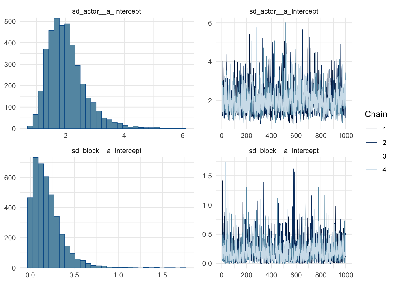
scale reduction factor on split chains (at convergence, Rhat = 1).

plot(m3)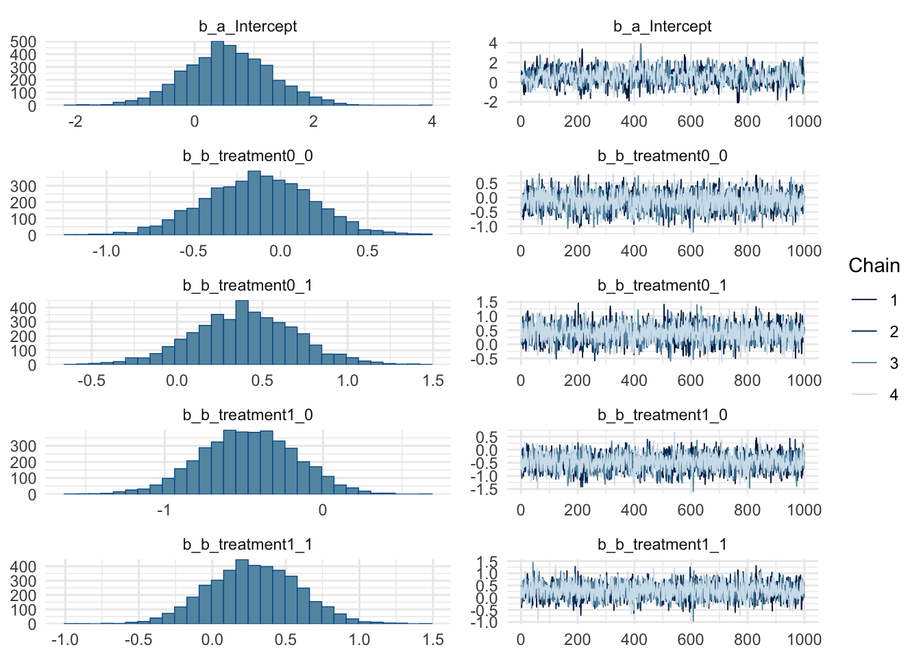

Python

az.summary(chimp_model_trace)

              mean     sd  hdi_3%  hdi_97%  ...  mcse_sd  ess_bulk  ess_tail  r_hat
a_bar        0.606  0.734  -0.848    1.948  ...    0.017     851.0    1173.0   1.00
z[1]        -0.528  0.398  -1.287    0.203  ...    0.008     738.0    1212.0   1.01
z[2]         2.109  0.627   0.932    3.247  ...    0.008    2010.0    2767.0   1.00
z[3]        -0.694  0.419  -1.503    0.057  ...    0.008     768.0    1459.0   1.00
z[4]        -0.693  0.412  -1.421    0.110  ...    0.008     745.0    1361.0   1.01
z[5]        -0.527  0.396  -1.248    0.222  ...    0.007     759.0    1650.0   1.01
z[6]        -0.017  0.365  -0.728    0.642  ...    0.007     839.0    1396.0   1.00
z[7]         0.814  0.442  -0.013    1.646  ...    0.007    1291.0    2104.0   1.00
x[1]        -0.708  0.865  -2.306    0.976  ...    0.015    3640.0    2647.0   1.00
x[2]         0.144  0.840  -1.450    1.733  ...    0.015    4311.0    2651.0   1.00
x[3]         0.210  0.846  -1.457    1.716  ...    0.015    3920.0    2498.0   1.00
x[4]         0.041  0.858  -1.559    1.702  ...    0.015    4443.0    2894.0   1.00
x[5]        -0.149  0.865  -1.808    1.530  ...    0.016    4171.0    2663.0   1.00
x[6]         0.469  0.851  -1.180    2.054  ...    0.015    3546.0    2645.0   1.00
beta[0_0]   -0.128  0.303  -0.676    0.452  ...    0.005    2071.0    2868.0   1.00
beta[0_1]    0.397  0.299  -0.161    0.962  ...    0.005    2016.0    2447.0   1.00
beta[1_0]   -0.478  0.298  -1.006    0.088  ...    0.004    2265.0    2552.0   1.00
beta[1_1]    0.280  0.302  -0.245    0.871  ...    0.004    1938.0    2304.0   1.00
sigma_a      2.004  0.656   0.981    3.238  ...    0.017    1034.0    2144.0   1.00
sigma_gamma  0.211  0.174   0.000    0.503  ...    0.005    1427.0    1835.0   1.00

[20 rows x 9 columns]

Check the forest plots, i.e., posterior coefficient plots:

R

m3 %>% mcmc_intervals(regex_pars = "^b_.*")
m3 %>% mcmc_areas(regex_pars = "^b_.*")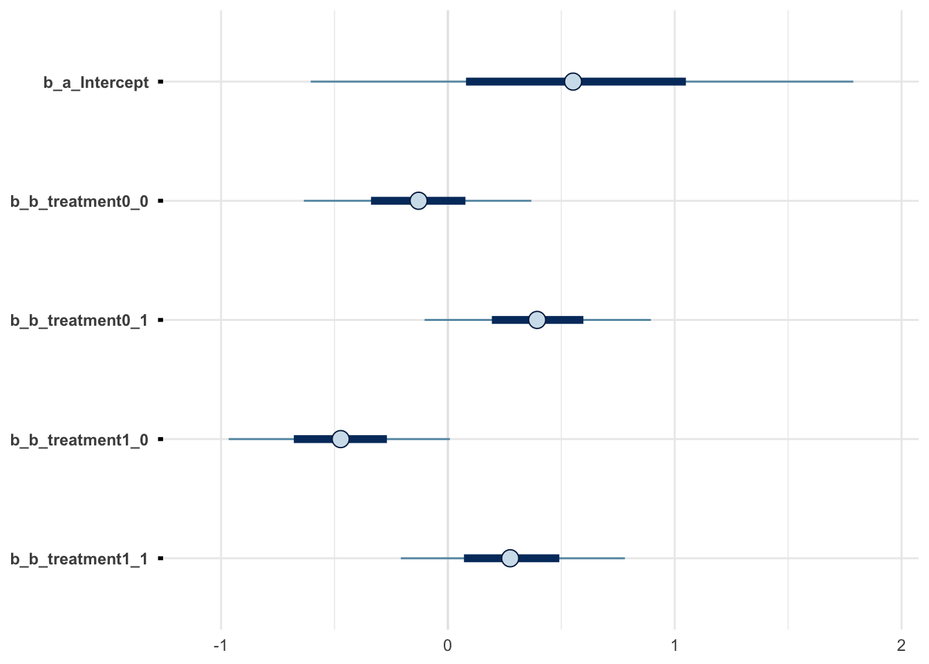

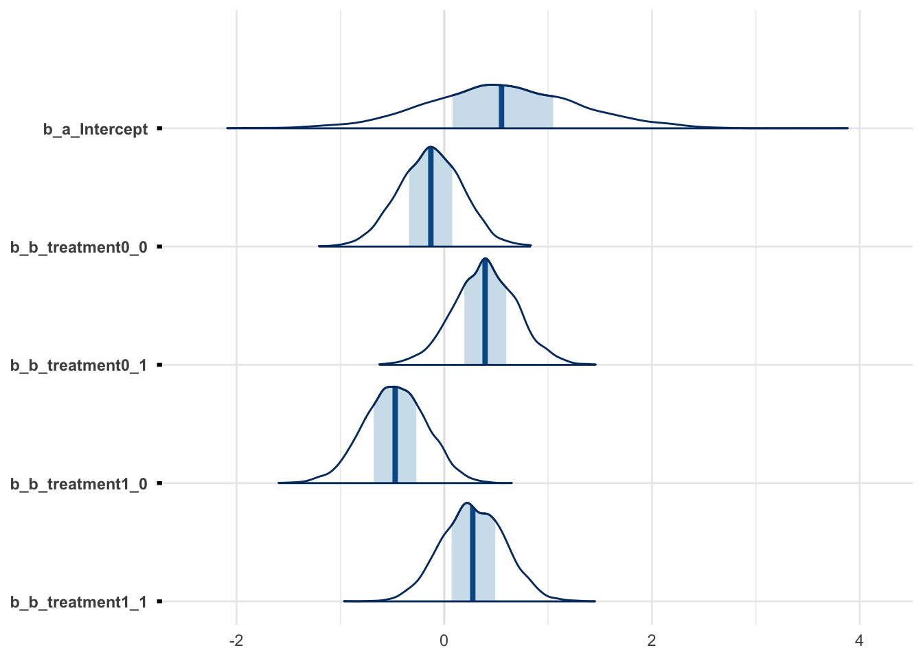
Python

az.plot_forest(chimp_model_trace, kind='forestplot', combined=True, hdi_prob=0.95)
az.plot_forest(chimp_model_trace, kind='ridgeplot', combined=True, hdi_prob=0.95)

array([<Axes: title={'center': '95.0% HDI'}>], dtype=object)

array([<Axes: >], dtype=object)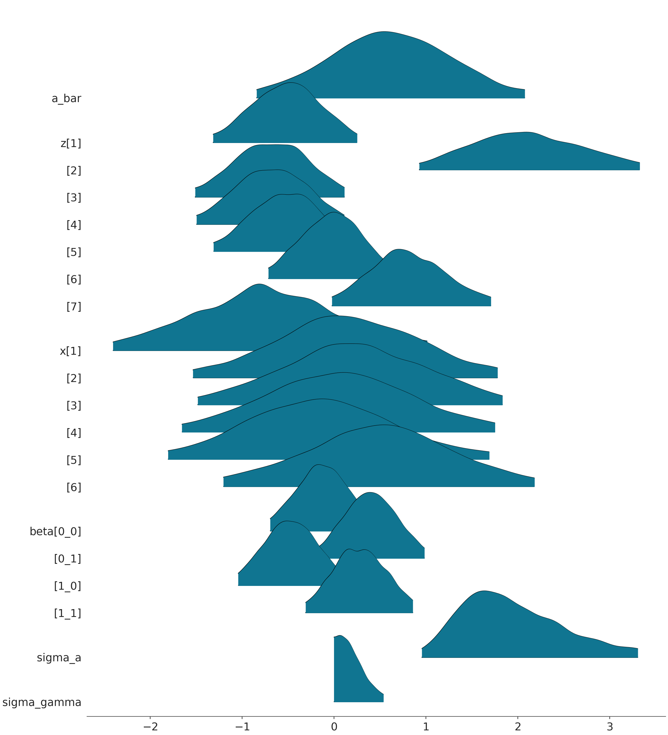

Perform a posterior predictive check:

R

pp_check(m3, ndraws = 100)
pp_check(m3, ndraws = 100, type="ecdf_overlay")
pp_check(m3, ndraws = 100, type="pit_ecdf")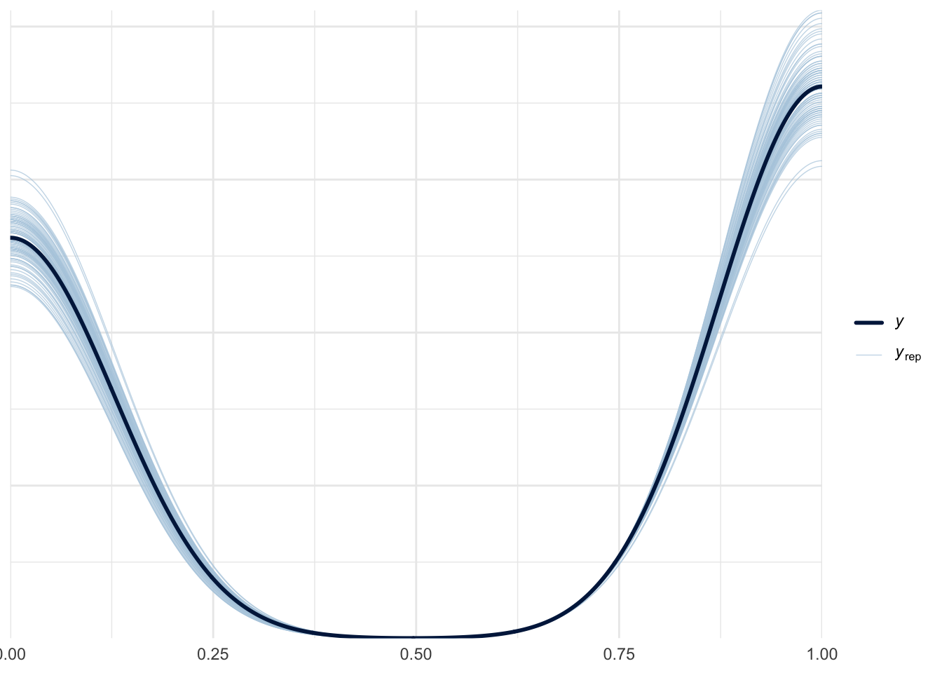

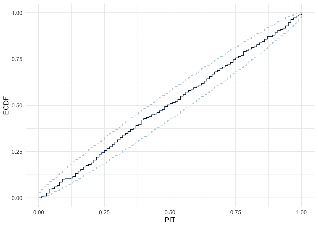
Python

azp.plot_ppc_dist(chimp_model_trace, group="posterior_predictive", num_samples=100)

<string>:1: UserWarning: Detected at least one discrete variable.
Consider using plot_ppc variants specific for discrete data, such as plot_ppc_pava or plot_ppc_rootogram.
<arviz_plots.plot_collection.PlotCollection object at 0x14795cb00>