Plotting with PyMC and Arviz

NoteTLDR

This post is about trying to answer a simple question: to what extent does existing functionalities of pymc and arviz implement what can be done in tidybayes …?

Trying to implement the examples here.

import arviz as az 
import pandas as pd 
import pymc as pm 
import numpy as np 
import matplotlib.pyplot as plt
az.style.use("arviz-docgrid")

RANDOM_SEED = 5
rng = np.random.default_rng(RANDOM_SEED)
n = 10
n_condition = 5
ABC = pd.DataFrame(rng.normal([0, 1, 2, 1, -1], scale=0.5, size=(n, n_condition))).set_axis(['A', 'B', 'C', 'D', 'E'], axis='columns')
ABC = pd.melt(ABC)

A snapshot of the data looks like this:

ABC.head(10)

	variable	value
0	A	-0.400966
1	A	0.054853
2	A	0.136384
3	A	-0.866067
4	A	-0.356657
5	A	0.414928
6	A	-0.644709
7	A	-0.198095
8	A	0.585148
9	A	0.016529

We can try to plot is as follows:

fig, ax = plt.subplots()
ax.scatter(data=ABC, x = "value", y = "variable")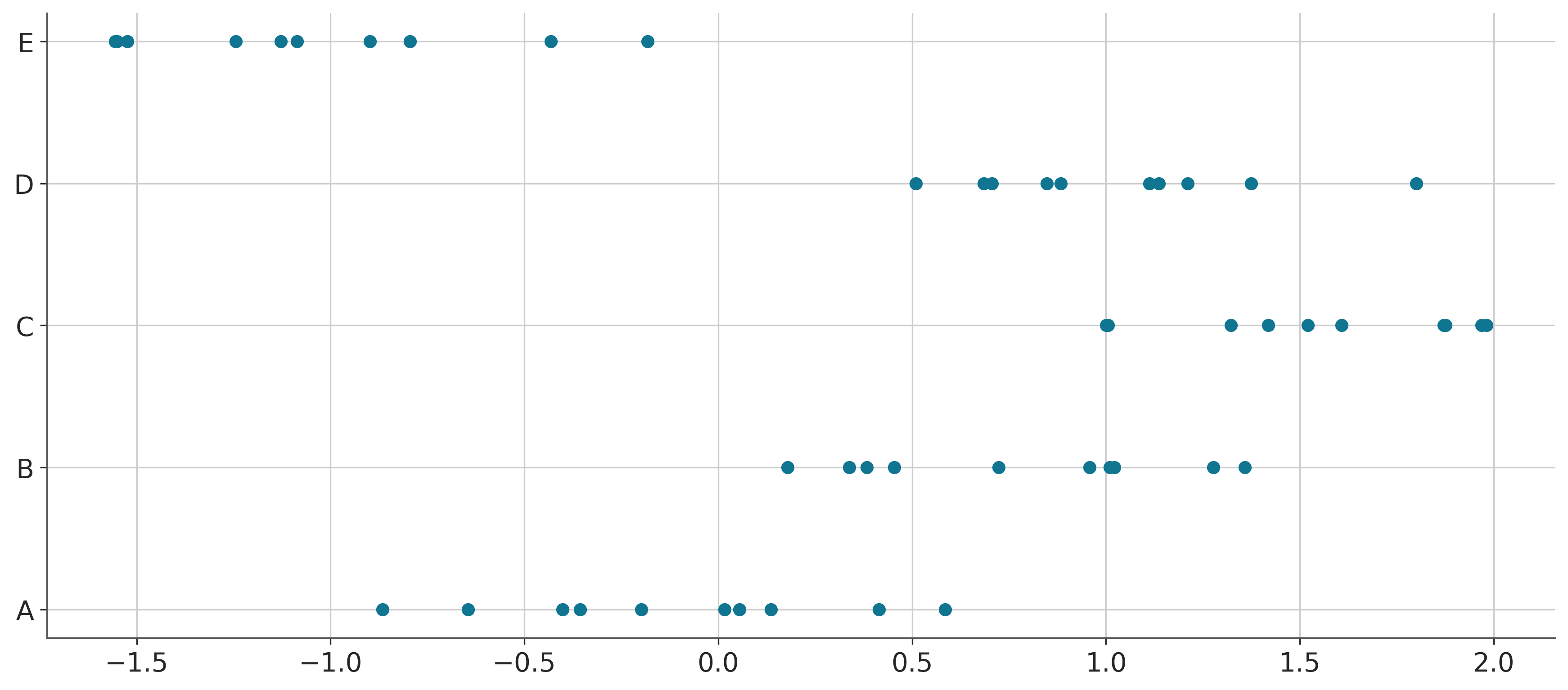

Model

We can fit a hierarchical model with shrinkage towards a global mean. The mathematical formulation is as follows:

\[ \begin{align} \texttt{value} &\sim \mathcal{N}(\alpha_{\text{variable}[i]}, \sigma) \\ \alpha_j &\sim \mathcal{N}(\bar{\alpha}, \sigma_\alpha), j \in [5] \\ \bar{\alpha} &\sim \mathcal{N}(0, 1) \\ \sigma_\alpha &\sim \text{student-t}^+(3, 0, 1) \\ \sigma &\sim \text{student-t}^+(3, 0, 1) \\ \end{align} \]

var_idx, var_value = pd.factorize(ABC['variable'])
coords = {
    'var': var_value
}

with pm.Model(coords=coords) as ABC_model:
    # priors and hyperpriors 
    alpha_bar = pm.Normal("alpha_bar", 0, 1)
    sigma_alpha = pm.HalfStudentT("sigma_alpha", nu=3, sigma=1)
    sigma = pm.HalfStudentT("sigma", nu=3, sigma=1)
    # likelihood ...? 
    alpha = pm.Normal("alpha", alpha_bar, sigma_alpha, dims="var")
    y_obs = pm.Normal("y_obs", mu=alpha[var_idx],sigma=sigma,observed=ABC['value'])

with ABC_model:
    idata = pm.sample(progressbar=False)

Initializing NUTS using jitter+adapt_diag...
Multiprocess sampling (4 chains in 4 jobs)
NUTS: [alpha_bar, sigma_alpha, sigma, alpha]
Sampling 4 chains for 1_000 tune and 1_000 draw iterations (4_000 + 4_000 draws total) took 19 seconds.

Note that in some of the tutorials, they refer to this as idata, perhaps a shorthand for the InferenceData object¹. In some other tutorials you would see this being referred to as XXXX_trace. Put simply, it is a container for groups of data.

¹ See official document for more details

idata

[autoreload of cutils_ext failed: Traceback (most recent call last):
  File "/Users/shenglong/Downloads/mika-long.github.io/.venv/lib/python3.13/site-packages/IPython/extensions/autoreload.py", line 325, in check
    superreload(m, reload, self.old_objects)
    ~~~~~~~~~~~^^^^^^^^^^^^^^^^^^^^^^^^^^^^^
  File "/Users/shenglong/Downloads/mika-long.github.io/.venv/lib/python3.13/site-packages/IPython/extensions/autoreload.py", line 580, in superreload
    module = reload(module)
  File "/Users/shenglong/.local/share/uv/python/cpython-3.13.9-macos-x86_64-none/lib/python3.13/importlib/__init__.py", line 128, in reload
    raise ModuleNotFoundError(f"spec not found for the module {name!r}", name=name)
ModuleNotFoundError: spec not found for the module 'cutils_ext'
]

arviz.InferenceData

• posterior

  <xarray.Dataset> Size: 264kB
  Dimensions:      (chain: 4, draw: 1000, var: 5)
  Coordinates:
    * chain        (chain) int64 32B 0 1 2 3
    * draw         (draw) int64 8kB 0 1 2 3 4 5 6 ... 993 994 995 996 997 998 999
    * var          (var) <U1 20B 'A' 'B' 'C' 'D' 'E'
  Data variables:
      alpha_bar    (chain, draw) float64 32kB 0.7988 0.7276 ... 0.4716 0.5919
      alpha        (chain, draw, var) float64 160kB 0.1649 0.8276 ... -1.001
      sigma_alpha  (chain, draw) float64 32kB 1.037 0.8986 0.7145 ... 1.314 0.7436
      sigma        (chain, draw) float64 32kB 0.3592 0.3608 ... 0.4625 0.3943
  Attributes:
      created_at:                 2025-12-18T22:07:06.287062+00:00
      arviz_version:              0.22.0
      inference_library:          pymc
      inference_library_version:  5.26.1
      sampling_time:              19.43943190574646
      tuning_steps:               1000

  xarray.Dataset

  • Dimensions:
    • chain: 4
    • draw: 1000
    • var: 5
  • Coordinates: (3)
    • chain
      (chain)
      int64
      0 1 2 3

      array([0, 1, 2, 3])

    • draw
      (draw)
      int64
      0 1 2 3 4 5 ... 995 996 997 998 999

      array([  0,   1,   2, ..., 997, 998, 999], shape=(1000,))

    • var
      (var)
      <U1
      'A' 'B' 'C' 'D' 'E'

      array(['A', 'B', 'C', 'D', 'E'], dtype='<U1')

  • Data variables: (4)
    • alpha_bar
      (chain, draw)
      float64
      0.7988 0.7276 ... 0.4716 0.5919

      array([[ 0.79879505,  0.72763475,  0.16616771, ..., -0.05006245,
               0.97315054, -0.67359004],
             [ 0.25249654,  0.2949005 ,  0.75311831, ..., -0.19206091,
               0.31462727,  0.37120262],
             [ 0.39568263,  0.46194458,  0.26003411, ...,  0.12332643,
               0.84393644, -0.19102742],
             [-0.0482245 ,  0.69851382,  0.54261485, ...,  0.21328792,
               0.47155153,  0.59190893]], shape=(4, 1000))

    • alpha
      (chain, draw, var)
      float64
      0.1649 0.8276 ... 0.8025 -1.001

      array([[[ 0.16487165,  0.82757603,  1.33422912,  0.95476705,
               -1.0322008 ],
              [ 0.07498675,  0.73138083,  1.52969247,  0.94640557,
               -1.03140938],
              [-0.11785607,  0.82427246,  1.52722905,  0.84256238,
               -1.13230676],
              ...,
              [-0.25830468,  0.70464512,  1.55445139,  1.02158926,
               -0.976952  ],
              [ 0.01124427,  0.9136963 ,  1.58118106,  1.08446858,
               -1.10788442],
              [-0.17204023,  0.71743021,  1.53025697,  0.88352464,
               -1.05506396]],
      
             [[-0.07828711,  0.77778781,  1.38530081,  1.30921337,
               -1.00643598],
              [-0.09809062,  0.92838083,  1.73418213,  1.30021465,
               -1.3547735 ],
              [-0.13145484,  0.76418426,  1.4554861 ,  1.24992397,
               -1.38936962],
      ...
              [-0.03656806,  0.79468535,  1.51641693,  0.92972396,
               -1.00529164],
              [-0.11302808,  0.74128492,  1.44604953,  1.07519885,
               -1.1492126 ],
              [-0.13884015,  0.80190369,  1.917893  ,  1.23285788,
               -1.0574313 ]],
      
             [[-0.11377738,  0.62382733,  1.43905909,  1.05863478,
               -0.99423062],
              [-0.07375993,  0.91278005,  1.64482255,  0.96034864,
               -0.98040235],
              [-0.04604509,  0.98042539,  1.48920905,  0.93903715,
               -1.2350581 ],
              ...,
              [ 0.04515829,  0.72148309,  1.5597229 ,  0.80576234,
               -1.01397494],
              [-0.2400069 ,  0.78463836,  1.51072601,  1.21668376,
               -0.95044114],
              [ 0.03505762,  0.66224036,  1.59119483,  0.80247834,
               -1.00120101]]], shape=(4, 1000, 5))

    • sigma_alpha
      (chain, draw)
      float64
      1.037 0.8986 ... 1.314 0.7436

      array([[1.03672796, 0.89855225, 0.71449234, ..., 1.56618828, 0.80322024,
              1.49290799],
             [0.65838449, 0.9798981 , 0.92754032, ..., 0.79425787, 0.90072488,
              0.67043663],
             [0.52904727, 1.8858211 , 0.71874636, ..., 0.84054065, 1.20098322,
              1.1907602 ],
             [0.62832242, 1.30280021, 1.46639108, ..., 0.66210809, 1.31417977,
              0.74358099]], shape=(4, 1000))

    • sigma
      (chain, draw)
      float64
      0.3592 0.3608 ... 0.4625 0.3943

      array([[0.35915039, 0.36080482, 0.39183955, ..., 0.42584479, 0.40403831,
              0.46403356],
             [0.52985762, 0.40589291, 0.53141016, ..., 0.41740445, 0.46089893,
              0.49593286],
             [0.3901418 , 0.43435049, 0.42924281, ..., 0.38836549, 0.43028774,
              0.47142696],
             [0.37349684, 0.49491954, 0.50273825, ..., 0.37883421, 0.4625165 ,
              0.39425398]], shape=(4, 1000))

  • Attributes: (6)

    created_at :

    2025-12-18T22:07:06.287062+00:00

    arviz_version :

    0.22.0

    inference_library :

    pymc

    inference_library_version :

    5.26.1

    sampling_time :

    19.43943190574646

    tuning_steps :

    1000

  
  
• sample_stats

  <xarray.Dataset> Size: 528kB
  Dimensions:                (chain: 4, draw: 1000)
  Coordinates:
    * chain                  (chain) int64 32B 0 1 2 3
    * draw                   (draw) int64 8kB 0 1 2 3 4 5 ... 995 996 997 998 999
  Data variables: (12/18)
      tree_depth             (chain, draw) int64 32kB 3 2 2 3 3 3 ... 3 2 3 3 2 2
      process_time_diff      (chain, draw) float64 32kB 0.000797 ... 0.001032
      index_in_trajectory    (chain, draw) int64 32kB 4 -1 -2 2 6 ... -2 -3 4 3 3
      n_steps                (chain, draw) float64 32kB 7.0 3.0 3.0 ... 3.0 3.0
      reached_max_treedepth  (chain, draw) bool 4kB False False ... False False
      largest_eigval         (chain, draw) float64 32kB nan nan nan ... nan nan
      ...                     ...
      perf_counter_start     (chain, draw) float64 32kB 1.229e+05 ... 1.229e+05
      acceptance_rate        (chain, draw) float64 32kB 0.9817 1.0 ... 0.8479
      energy_error           (chain, draw) float64 32kB 0.1371 -0.9504 ... -0.2354
      max_energy_error       (chain, draw) float64 32kB -0.5344 -0.9504 ... 0.6091
      step_size              (chain, draw) float64 32kB 0.5511 0.5511 ... 1.152
      step_size_bar          (chain, draw) float64 32kB 0.7092 0.7092 ... 0.8041
  Attributes:
      created_at:                 2025-12-18T22:07:06.348796+00:00
      arviz_version:              0.22.0
      inference_library:          pymc
      inference_library_version:  5.26.1
      sampling_time:              19.43943190574646
      tuning_steps:               1000

  xarray.Dataset

  • Dimensions:
    • chain: 4
    • draw: 1000
  • Coordinates: (2)
    • chain
      (chain)
      int64
      0 1 2 3

      array([0, 1, 2, 3])

    • draw
      (draw)
      int64
      0 1 2 3 4 5 ... 995 996 997 998 999

      array([  0,   1,   2, ..., 997, 998, 999], shape=(1000,))

  • Data variables: (18)
    • tree_depth
      (chain, draw)
      int64
      3 2 2 3 3 3 2 3 ... 3 2 3 2 3 3 2 2

      array([[3, 2, 2, ..., 3, 3, 3],
             [3, 3, 3, ..., 3, 3, 3],
             [2, 2, 3, ..., 2, 2, 2],
             [2, 3, 3, ..., 3, 2, 2]], shape=(4, 1000))

    • process_time_diff
      (chain, draw)
      float64
      0.000797 0.000383 ... 0.001032

      array([[0.000797, 0.000383, 0.000418, ..., 0.000714, 0.000845, 0.000708],
             [0.000984, 0.00104 , 0.001235, ..., 0.00073 , 0.00073 , 0.00071 ],
             [0.000382, 0.000419, 0.000736, ..., 0.000432, 0.000513, 0.000563],
             [0.000373, 0.000728, 0.001385, ..., 0.001586, 0.000999, 0.001032]],
            shape=(4, 1000))

    • index_in_trajectory
      (chain, draw)
      int64
      4 -1 -2 2 6 2 -2 ... 7 -2 -3 4 3 3

      array([[ 4, -1, -2, ...,  4, -4,  3],
             [ 5, -6,  7, ..., -1,  1,  1],
             [ 0, -3,  4, ...,  0, -3, -3],
             [-1, -4,  1, ...,  4,  3,  3]], shape=(4, 1000))

    • n_steps
      (chain, draw)
      float64
      7.0 3.0 3.0 7.0 ... 7.0 7.0 3.0 3.0

      array([[7., 3., 3., ..., 7., 7., 7.],
             [7., 7., 7., ..., 7., 7., 7.],
             [3., 3., 7., ..., 3., 3., 3.],
             [3., 7., 7., ..., 7., 3., 3.]], shape=(4, 1000))

    • reached_max_treedepth
      (chain, draw)
      bool
      False False False ... False False

      array([[False, False, False, ..., False, False, False],
             [False, False, False, ..., False, False, False],
             [False, False, False, ..., False, False, False],
             [False, False, False, ..., False, False, False]], shape=(4, 1000))

    • largest_eigval
      (chain, draw)
      float64
      nan nan nan nan ... nan nan nan nan

      array([[nan, nan, nan, ..., nan, nan, nan],
             [nan, nan, nan, ..., nan, nan, nan],
             [nan, nan, nan, ..., nan, nan, nan],
             [nan, nan, nan, ..., nan, nan, nan]], shape=(4, 1000))

    • divergences
      (chain, draw)
      int64
      0 0 0 0 0 0 0 0 ... 0 0 0 0 0 0 0 0

      array([[0, 0, 0, ..., 0, 0, 0],
             [0, 0, 0, ..., 0, 0, 0],
             [0, 0, 0, ..., 0, 0, 0],
             [0, 0, 0, ..., 0, 0, 0]], shape=(4, 1000))

    • energy
      (chain, draw)
      float64
      44.12 42.14 40.45 ... 40.6 42.04

      array([[44.11999358, 42.14067237, 40.44714286, ..., 41.71500086,
              40.80141104, 40.57003386],
             [44.22337106, 45.49841608, 46.80329307, ..., 43.98499662,
              40.09734042, 40.87232229],
             [44.35259949, 41.20855321, 41.59342702, ..., 41.67505082,
              39.89664177, 43.58927654],
             [40.0447229 , 41.3907074 , 42.70211086, ..., 44.89368373,
              40.60135264, 42.04476507]], shape=(4, 1000))

    • lp
      (chain, draw)
      float64
      -41.37 -37.62 ... -37.79 -37.96

      array([[-41.36768433, -37.61669089, -37.12016517, ..., -37.09129342,
              -38.00552631, -38.80126266],
             [-41.00439614, -43.02991079, -42.65772859, ..., -39.36388076,
              -36.77093313, -38.08148589],
             [-39.19669511, -37.69602526, -36.47985897, ..., -35.73725033,
              -36.85572906, -41.6000285 ],
             [-38.30529551, -38.32060245, -40.16437261, ..., -38.34492319,
              -37.79167984, -37.95596749]], shape=(4, 1000))

    • perf_counter_diff
      (chain, draw)
      float64
      0.0007976 0.000383 ... 0.00131

      array([[0.00079756, 0.00038301, 0.00041667, ..., 0.00071286, 0.00084403,
              0.00070627],
             [0.00105956, 0.00105258, 0.00125841, ..., 0.00072913, 0.00073008,
              0.00070991],
             [0.00038216, 0.0004182 , 0.0007355 , ..., 0.00043181, 0.00051792,
              0.00058225],
             [0.00037279, 0.00072753, 0.00158695, ..., 0.00253081, 0.0011158 ,
              0.00131013]], shape=(4, 1000))

    • diverging
      (chain, draw)
      bool
      False False False ... False False

      array([[False, False, False, ..., False, False, False],
             [False, False, False, ..., False, False, False],
             [False, False, False, ..., False, False, False],
             [False, False, False, ..., False, False, False]], shape=(4, 1000))

    • smallest_eigval
      (chain, draw)
      float64
      nan nan nan nan ... nan nan nan nan

      array([[nan, nan, nan, ..., nan, nan, nan],
             [nan, nan, nan, ..., nan, nan, nan],
             [nan, nan, nan, ..., nan, nan, nan],
             [nan, nan, nan, ..., nan, nan, nan]], shape=(4, 1000))

    • perf_counter_start
      (chain, draw)
      float64
      1.229e+05 1.229e+05 ... 1.229e+05

      array([[122934.03717517, 122934.0381256 , 122934.03866246, ...,
              122935.10795202, 122935.1087929 , 122935.10977299],
             [122934.07734157, 122934.07858957, 122934.08001443, ...,
              122935.16853006, 122935.16939254, 122935.17025179],
             [122934.05681384, 122934.05733257, 122934.05788432, ...,
              122935.07279388, 122935.07338315, 122935.07413444],
             [122935.36613427, 122935.36664097, 122935.36750012, ...,
              122936.35222003, 122936.35531774, 122936.35674233]],
            shape=(4, 1000))

    • acceptance_rate
      (chain, draw)
      float64
      0.9817 1.0 0.8836 ... 0.9322 0.8479

      array([[0.98169298, 1.        , 0.88362648, ..., 0.80311617, 0.8578346 ,
              0.84429589],
             [0.50468484, 0.91838947, 0.98324889, ..., 0.68691957, 1.        ,
              0.78884007],
             [0.01634626, 1.        , 0.78599644, ..., 0.47934719, 0.50487524,
              0.59239985],
             [0.58363336, 1.        , 0.85094789, ..., 0.75324596, 0.93217334,
              0.8479473 ]], shape=(4, 1000))

    • energy_error
      (chain, draw)
      float64
      0.1371 -0.9504 ... 0.04509 -0.2354

      array([[ 0.1371369 , -0.95039891, -0.09301714, ..., -0.16316772,
               0.29807756,  0.20501956],
             [ 0.60901932,  0.32907349, -0.28207176, ...,  0.65662321,
              -0.67146844,  0.24485943],
             [ 0.        , -0.30180116, -0.40854078, ...,  0.        ,
               0.55672924,  0.58655594],
             [ 0.54847462, -0.20170781,  0.18224042, ..., -1.11827008,
               0.04509219, -0.23538491]], shape=(4, 1000))

    • max_energy_error
      (chain, draw)
      float64
      -0.5344 -0.9504 ... 0.1736 0.6091

      array([[-0.53440217, -0.95039891,  0.41998121, ...,  0.64532742,
              -0.32900204,  0.35901684],
             [ 0.98392794, -0.66605619, -0.95092064, ...,  0.65662321,
              -0.68902882,  0.39509102],
             [ 5.25682031, -0.42914533,  0.54249493, ...,  0.80356013,
               1.15836484,  0.63100665],
             [ 0.6870315 , -0.60186569,  0.61948124, ...,  2.42378742,
               0.17362667,  0.60909669]], shape=(4, 1000))

    • step_size
      (chain, draw)
      float64
      0.5511 0.5511 ... 1.152 1.152

      array([[0.55107601, 0.55107601, 0.55107601, ..., 0.55107601, 0.55107601,
              0.55107601],
             [0.69157915, 0.69157915, 0.69157915, ..., 0.69157915, 0.69157915,
              0.69157915],
             [0.81780947, 0.81780947, 0.81780947, ..., 0.81780947, 0.81780947,
              0.81780947],
             [1.15236493, 1.15236493, 1.15236493, ..., 1.15236493, 1.15236493,
              1.15236493]], shape=(4, 1000))

    • step_size_bar
      (chain, draw)
      float64
      0.7092 0.7092 ... 0.8041 0.8041

      array([[0.70924133, 0.70924133, 0.70924133, ..., 0.70924133, 0.70924133,
              0.70924133],
             [0.73812004, 0.73812004, 0.73812004, ..., 0.73812004, 0.73812004,
              0.73812004],
             [0.70855132, 0.70855132, 0.70855132, ..., 0.70855132, 0.70855132,
              0.70855132],
             [0.80413936, 0.80413936, 0.80413936, ..., 0.80413936, 0.80413936,
              0.80413936]], shape=(4, 1000))

  • Attributes: (6)

    created_at :

    2025-12-18T22:07:06.348796+00:00

    arviz_version :

    0.22.0

    inference_library :

    pymc

    inference_library_version :

    5.26.1

    sampling_time :

    19.43943190574646

    tuning_steps :

    1000

  
  
• observed_data

  <xarray.Dataset> Size: 800B
  Dimensions:      (y_obs_dim_0: 50)
  Coordinates:
    * y_obs_dim_0  (y_obs_dim_0) int64 400B 0 1 2 3 4 5 6 ... 43 44 45 46 47 48 49
  Data variables:
      y_obs        (y_obs_dim_0) float64 400B -0.401 0.05485 ... -1.551 -1.128
  Attributes:
      created_at:                 2025-12-18T22:07:06.364057+00:00
      arviz_version:              0.22.0
      inference_library:          pymc
      inference_library_version:  5.26.1

  xarray.Dataset

  • Dimensions:
    • y_obs_dim_0: 50
  • Coordinates: (1)
    • y_obs_dim_0
      (y_obs_dim_0)
      int64
      0 1 2 3 4 5 6 ... 44 45 46 47 48 49

      array([ 0,  1,  2,  3,  4,  5,  6,  7,  8,  9, 10, 11, 12, 13, 14, 15, 16, 17,
             18, 19, 20, 21, 22, 23, 24, 25, 26, 27, 28, 29, 30, 31, 32, 33, 34, 35,
             36, 37, 38, 39, 40, 41, 42, 43, 44, 45, 46, 47, 48, 49])

  • Data variables: (1)
    • y_obs
      (y_obs_dim_0)
      float64
      -0.401 0.05485 ... -1.551 -1.128

      array([-0.40096571,  0.0548532 ,  0.13638439, -0.86606742, -0.35665669,
              0.41492765, -0.64470937, -0.19809517,  0.58514805,  0.01652861,
              0.3378205 ,  0.72367634,  0.38333567,  0.9581519 ,  1.27668924,
              0.17848831,  1.0103452 ,  0.45433555,  1.35829383,  1.021816  ,
              1.87581919,  1.60760982,  1.5208674 ,  1.41838701,  1.96845701,
              1.87163494,  1.98105713,  1.32239563,  1.00109165,  1.00578511,
              1.21022262,  1.37437289,  1.80000954,  0.68535595,  0.70528437,
              0.50962632,  0.84783112,  1.11239287,  1.13606443,  0.88328874,
             -0.43197673, -0.18260848, -0.89855878, -1.24400291, -0.79518109,
             -1.08657761, -1.52396325, -1.55467497, -1.55085831, -1.12789502])

  • Attributes: (4)

    created_at :

    2025-12-18T22:07:06.364057+00:00

    arviz_version :

    0.22.0

    inference_library :

    pymc

    inference_library_version :

    5.26.1

  
  

In this case, the InferenceData² has contains three “datasets”: posterior, sample_stats, and observed_data.

² In the example in the original documentation, it also has posterior_predictive and prior

We could access the posterior draws simply by directly referencing it:

print(idata.posterior)
print(type(idata.posterior))

<xarray.Dataset> Size: 264kB
Dimensions:      (chain: 4, draw: 1000, var: 5)
Coordinates:
  * chain        (chain) int64 32B 0 1 2 3
  * draw         (draw) int64 8kB 0 1 2 3 4 5 6 ... 993 994 995 996 997 998 999
  * var          (var) <U1 20B 'A' 'B' 'C' 'D' 'E'
Data variables:
    alpha_bar    (chain, draw) float64 32kB 0.7988 0.7276 ... 0.4716 0.5919
    alpha        (chain, draw, var) float64 160kB 0.1649 0.8276 ... -1.001
    sigma_alpha  (chain, draw) float64 32kB 1.037 0.8986 0.7145 ... 1.314 0.7436
    sigma        (chain, draw) float64 32kB 0.3592 0.3608 ... 0.4625 0.3943
Attributes:
    created_at:                 2025-12-18T22:07:06.287062+00:00
    arviz_version:              0.22.0
    inference_library:          pymc
    inference_library_version:  5.26.1
    sampling_time:              19.43943190574646
    tuning_steps:               1000
<class 'xarray.core.dataset.Dataset'>

Those who are more familiar with the tidy data format might find the above ways of indexing with coordinates and dimensions confusing. We could turn the Dataset into a DataFrame in tidy form³:

³ See reference documentation here

idata.posterior.to_dataframe().head(10)

			alpha_bar	alpha	sigma_alpha	sigma
chain	draw	var
0	0	A	0.798795	0.164872	1.036728	0.359150
		B	0.798795	0.827576	1.036728	0.359150
		C	0.798795	1.334229	1.036728	0.359150
		D	0.798795	0.954767	1.036728	0.359150
		E	0.798795	-1.032201	1.036728	0.359150
	1	A	0.727635	0.074987	0.898552	0.360805
		B	0.727635	0.731381	0.898552	0.360805
		C	0.727635	1.529692	0.898552	0.360805
		D	0.727635	0.946406	0.898552	0.360805
		E	0.727635	-1.031409	0.898552	0.360805

# save fitted posterior 
# giidata.to_netcdf("ABC_posterior.nc")

---

tidybayes provides functions such as median_qi() and mode_hdi() for calculating point summaries and intervals. Their equivalent in arviz are arviz_stats.eti and arviz.hdi.

print(az.hdi(idata, var_names=["alpha_bar", "sigma"], hdi_prob = 0.95).to_dataframe())

        alpha_bar     sigma
hdi                        
lower   -0.574370  0.346919
higher   1.308319  0.528288

import arviz_stats as avz 

avz.eti(idata, var_names=["alpha_bar", "sigma"], prob = 0.95).to_dataframe()

	alpha_bar	sigma
ci_bound
lower	-0.592632	0.352223
upper	1.290091	0.536236

We can also get a table of summary statistics with the arviz.summary function:

az.summary(idata, stat_focus="median", hdi_prob=0.95)

	median	mad	eti_2.5%	eti_97.5%	mcse_median	ess_median	ess_tail	r_hat
alpha_bar	0.367	0.306	-0.593	1.290	0.008	4272.107	2404.0	1.0
alpha[A]	-0.115	0.089	-0.385	0.152	0.002	5423.275	2903.0	1.0
alpha[B]	0.757	0.088	0.499	1.024	0.002	4692.825	3062.0	1.0
alpha[C]	1.530	0.089	1.265	1.806	0.002	5169.563	3147.0	1.0
alpha[D]	1.015	0.090	0.742	1.272	0.003	4640.295	2776.0	1.0
alpha[E]	-1.016	0.090	-1.284	-0.733	0.003	5131.215	3237.0	1.0
sigma_alpha	1.043	0.224	0.601	2.238	0.006	3460.928	2362.0	1.0
sigma	0.426	0.032	0.352	0.536	0.001	4113.274	3118.0	1.0

az.summary(idata, stat_focus="mean", hdi_prob=0.95)

	mean	sd	hdi_2.5%	hdi_97.5%	mcse_mean	mcse_sd	ess_bulk	ess_tail	r_hat
alpha_bar	0.359	0.477	-0.574	1.308	0.008	0.010	3632.0	2404.0	1.0
alpha[A]	-0.117	0.135	-0.364	0.170	0.002	0.002	5170.0	2903.0	1.0
alpha[B]	0.760	0.133	0.504	1.027	0.002	0.002	4871.0	3062.0	1.0
alpha[C]	1.532	0.137	1.269	1.810	0.002	0.002	5601.0	3147.0	1.0
alpha[D]	1.012	0.135	0.757	1.284	0.002	0.002	4985.0	2776.0	1.0
alpha[E]	-1.014	0.137	-1.266	-0.721	0.002	0.002	4918.0	3237.0	1.0
sigma_alpha	1.138	0.434	0.524	1.966	0.009	0.014	3212.0	2362.0	1.0
sigma	0.431	0.047	0.347	0.528	0.001	0.001	4120.0	3118.0	1.0

az.plot_forest(idata, combined=True, var_names=["alpha"], hdi_prob=0.95)

array([<Axes: title={'center': '95.0% HDI'}>], dtype=object)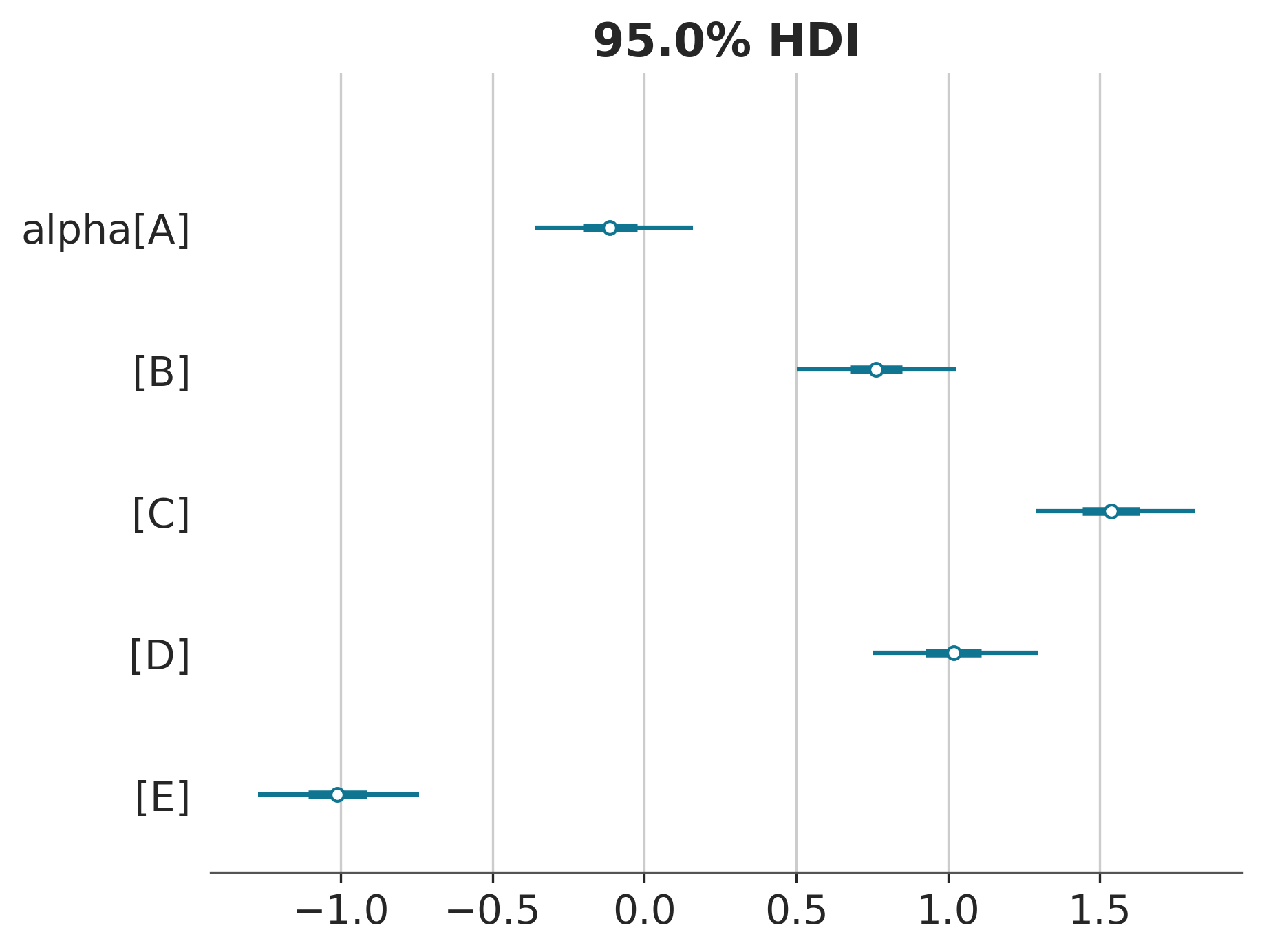

Intervals with densities

az.plot_forest(idata, combined=True, var_names=["alpha"], hdi_prob=0.95, kind="ridgeplot")

array([<Axes: >], dtype=object)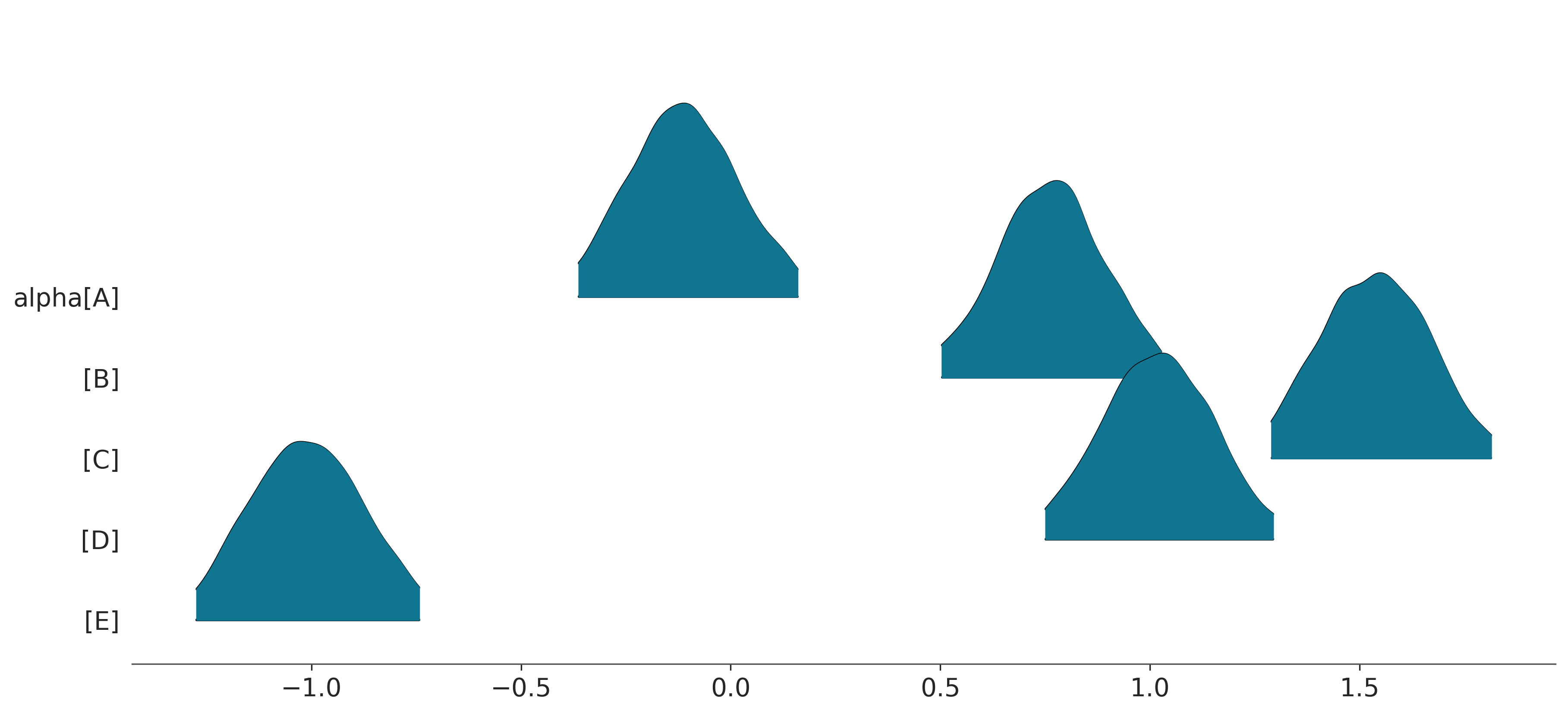

… yeah the above kind of looks ugly LOL … to actually reproduce the slabinterval geom one would need to do something else …

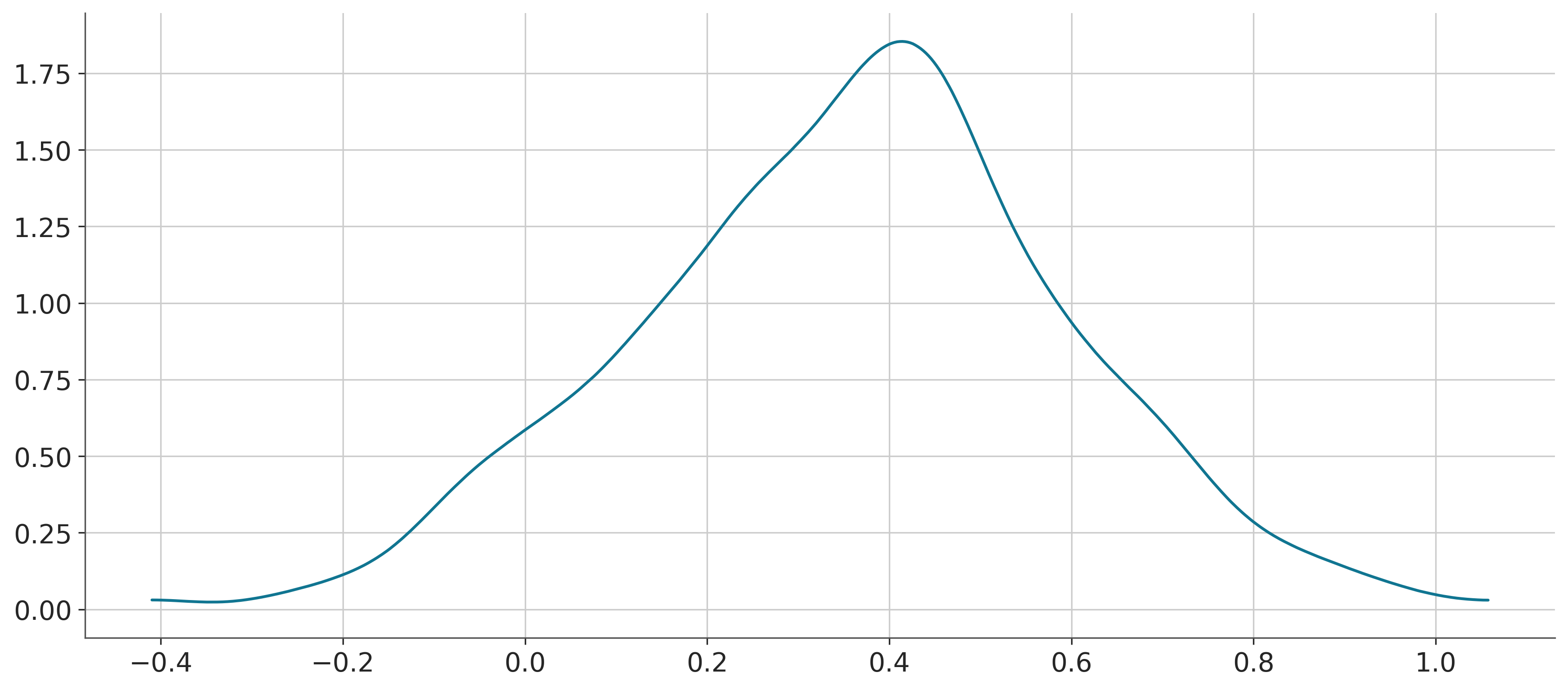
# TODO 

Posterior means and predictions

idata.posterior['alpha_bar'].mean()

<xarray.DataArray 'alpha_bar' ()> Size: 8B
array(0.3586002)

xarray.DataArray

'alpha_bar'

• 0.3586

  array(0.3586002)

az.plot_dist(idata.posterior['alpha_bar'].mean(dim="chain"))